A MODIFIED BIC TUNING PARAMETER SELECTOR FOR SICA-PENALIZED COX REGRESSION MODELS WITH DIVERGING DIMENSIONALITY

SHI Yue-yongJIAO Yu-lingYAN LiangCAO Yong-xiu

(1.School of Economics and Management,China University of Geosciences,Wuhan 430074,China)(2.School of Statistics and Mathematics,Zhongnan University of Economics and Law,Wuhan 430073,China)(3.Center for Resources and Environmental Economic Research,China University of Geosciences,Wuhan 430074,China)

A MODIFIED BIC TUNING PARAMETER SELECTOR FOR SICA-PENALIZED COX REGRESSION MODELS WITH DIVERGING DIMENSIONALITY

SHI Yue-yong1,3,JIAO Yu-ling2,YAN Liang1,CAO Yong-xiu2

(1.School of Economics and Management,China University of Geosciences,Wuhan 430074,China)(2.School of Statistics and Mathematics,Zhongnan University of Economics and Law,Wuhan 430073,China)(3.Center for Resources and Environmental Economic Research,China University of Geosciences,Wuhan 430074,China)

This paper proposes a modi fi ed BIC(Bayesian information criterion)tuning parameter selector for SICA-penalized Cox regression models with a diverging number of covariates.Under some regularity conditions,we prove the model selection consistency of the proposed method.Numerical results show that the proposed method performs better than the GCV(generalized crossvalidation)criterion.

Cox models;modi fi ed BIC;penalized likelihood;SICA penalty;smoothing quasi-Newton

1 Introduction

The commonly used Cox model[4]for survival data assumes that the hazard functionh(t|z)for the failure timeTassociated with covariates z=(z1,···,zd)Ttakes the form

wheretis the time,h0(t)is an arbitrary unspeci fi ed baseline Hazard function andβ=(β1,···,βd)Tis an unknown vector of regression coefficients.In this paper,we consider the following so-called SICA-penalized log partial likelihood(SPPL)problem

where

is the logarithm of the partial likelihood function,=min(Ti,Ci),δi=I(Ti≤Ci),Yi(t)=I(≥t),andTiandCiare the failure time and censoring time of subjecti(i=1,···,n),respectively;pλ,τ(βj)=λ(τ+1)|βj|/(|βj| +τ)is the SICA penalty function proposed by Lv and Fan[9],andλandτare two positive tuning(or regularization)parameters.In particular,λis the sparsity tuning parameter obtaining sparse solutions andτis the shape(or concavity)tuning parameter making SICA a bridge betweenL0(τ→0+)andL1(τ→∞),whereL0andL1admitpλ(βj)=λI(|βj|0)andpλ(βj)=λ|βj| ,respectively.ˆβ,which is dependent onλandτ,i.e.,=(λ,τ),is denoted as a SPPL estimator.

Although penalized likelihood methods can select variables and estimate coefficients simultaneously,their optimal properties heavily depend on an appropriate selection of the tuning parameters.Thus,an important issue in variable selection using penalized likelihood methods is the choice of tuning parameters.Some common used tuning parameter selection criteria are GCV[1,6,8,13],AIC[17]and BIC[14,15].

Shi et al.[12]proposed using the SPPL approach combined with a GCV tuning parameter selector for variable selection in Cox’s proportional hazards model with diverging dimensionality.As shown in Wang et al.[14,15]in the linear model case,it is known that GCV tends to over- fi t the true model and BIC can identify the true model consistently.Thus,when the primary goal is variable selection and identi fi cation of the true model,BIC may be preferred over GCV.In this paper,in the context of right-censored data,we modify the classical BIC to select tuning parameters for(1.2)and prove its consistency when the number of regression coefficients tends to in fi nity.Simulation studies are given to illustrate the performance of the proposed approach.

An outline for this paper is as follows.In Section 2,we fi rst describe the Modi fi ed BIC method for SPPL and then give theoretical results and corresponding proofs.The fi nite sample performance of the proposed method through simulation studies are demonstrated in Section 3.We conclude the paper with Section 4.

2 Modi fi ed BIC(MBIC)for SPPL

2.1 Methodology

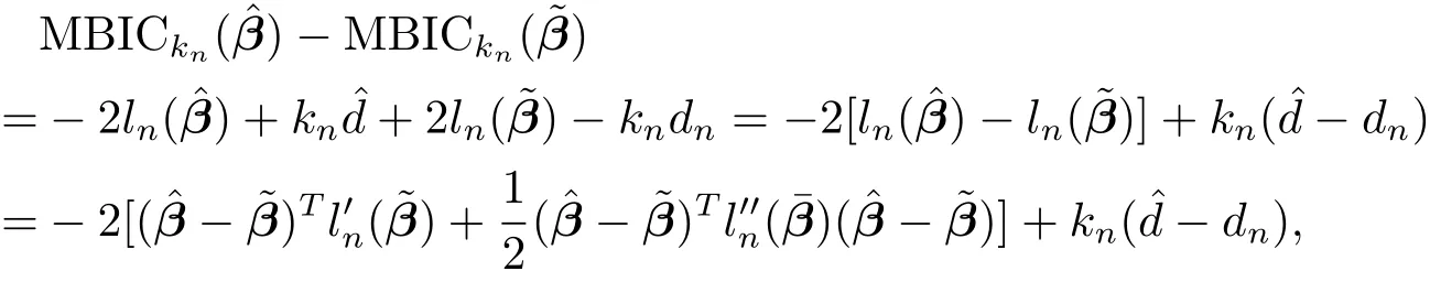
The ordinary BIC procedure is implemented by minimizing

2.2 Theoretical Results

Without loss of generality,we write the true parameter vector aswhereβ10consists of allsnonzero components andβ20consists of the remaining zero components.Correspondingly,we write the maximizer of(1.2)as.De fi ne.Hereafter,sometimes we usedn,sn,λnandτnrather thand,s,λandτto emphasize their dependence onn.The regularity conditions(C1)-(C7)in[12]are assumed in the following theoretical results.

Theorem 1(Existence of SPPL estimator)Under conditions(C1)-(C7)in[12],with probability tending to one,there exists a local maximizerofQn(β),defined in(1.2),such that,where‖·‖2is theL2norm on the Euclidean space.

Theorem 2(Oracle property)Under conditions(C1)-(C7)in[12],with probability tending to 1,the-consistent local maximizerin Theorem 1 must be such that

(ii)(Asymptotic normality)For any nonzero constantsn×1 vectorcnwith

in distribution,whereA11and Γ11consist of the fi rstsncolumns and rows ofA(β10,0)and Γ(β10,0)respectively,andA(β)and Γ(β)are defined in Appendix of[12].

Regularity conditions and detailed proofs for Theorem 1 and Theorem 2 can be found in Appendix of[12].We now present the main result on the selection consistency of the MBIC under conditions(C1)-(C7)in[12]and an extra condition

Suppose ΩR2.We defineand.In other words,Ω0,Ω-and Ω+are three subsets of Ω,in which the true,under fi tted and over fi tted models can be produced.It easily follows that Ω=Ω0∪Ω+∪Ω-(disjoint union)andbe the local maxima of SPPL described in Theorem 1.

Theorem 3Under conditions(C1)-(C8),

ProofSincekn＞log(n),without loss of generality,we assumekn＞1.We prove this theorem by considering two di ff erent cases,i.e.,under fi tting and over fi tting.

Case 1Under fi tted model,i.e.,,which meansargmaxln(β),namely,is the ordinary maximum partial likelihood estimator(MLE).By the second-order Taylor expansion of the log partial likelihood,we have

wherer=λmin{A(β0)}.Since,we have.Condition(C6)impliesρn/αn→ ∞.Together with,we have

and then we get

Next we considerI2.It easily follows that

By(2.5),(2.6))and condition(C8),we have

which yields

Thus we deduce that the minimum MBIC can not be selected from the under fi tted model.

Case 2Over fi tted model,i.e.,,which meansIn this case,we have.De fi nea vector with the same length ofandAccording to Theorem 1 and Theorem 2,we have,whereBy the de fi nition of MBIC,it follows that

which implies

Thus we deduce that the minimum MBIC can not be selected from the over fi tted model.

The results of Cases 1 and 2 complete the proof.

Remark 1Theorem 3 implies that ifis chosen to minimize MBIC with an appropriately chosenkn,thenis consistent for model selection.

3 Computation

3.1 Algorithm

We apply the smoothing quasi-Newton(SQN)method to optimizeQn(β)in(1.2).Since the SICA penalty function is singular at the origin,we fi rst smooth the objective function by replacing|βj| with,whereεis a small positive quantity.It follows thatwhenε→0.Then we maximize

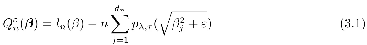
instead of maximizingQn(β)by using the DFP quasi-Newton method with backtracking linear search algorithm procedure(e.g.[11]).In practice,takingε=0.01 gives good results.The pseudo-code for our algorithmic implementation can be found in[12].More theoretical results about smoothing methods for nonsmooth and noconvex minimization can be found in[2,3].

Remark 2Like the LQA(local quadratic approximation)algorithm in[6],the sequenceβkobtained from SQN(DFP)may not be sparse for any fi xedkand hence is not directly suitable for variable selection.In practice,we setfor some sufficiently small tolerance levelε0,whereis thejth element ofβk.

3.2 Covariance Estimation

Following[12],we estimate the covariance matrix(i.e.,standard errors)for1(the nonvanishing component of)by using the sandwich formulae

3.3 Tuning Parameter Selection

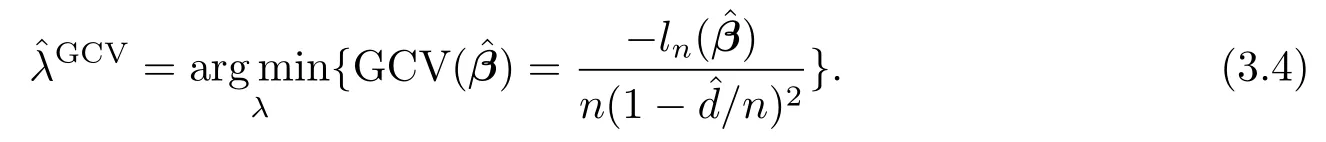
Numerical results suggest that the performance of SPPL estimator is robust to the choice ofτandτ=0.01 seems to give reasonable results in simulations,so we fi xτ=0.01 and concentrate on tuningλvia

where we choosekn=2log(n)in the numerical experiments.We compare the performance of SPPL-MBIC with SPPL-GCV which solves

In practice,we consider a range of values forλ：λmax=λ0＞···＞λG=0 for some positive numberλ0andG,whereλ0is an initial guess ofλ,supposedly large,andGis the number of grid points(we takeG=100 in our numerical experiments).

3.4 Simulation Study

In this subsection,we illustrate the fi nite sample properties of SPPL-MBIC with a simulated example and compare it with the SPPL-GCV method.All simulations are conducted using MATLAB codes.

We simulated 100 data sets from the exponential hazards model

whereβ0∈R8withβ01=0.5,β02=1,β03=-0.9,andβ0j=0,if1,2,3.Thusd=8 andd0=3.The 8 covariates z=(z1,···,z8)Tare marginally standard normal with pairwise correlations corr(zj,zk)=ρ|j-k|.We assume moderate correlation between the covariates by takingρ=0.5.Censoring times are generated from a uniform distribution U(0,r),whereris chosen to have approximately 25%censoring rate.Sample sizesn=150 and 200 are considered.

To evaluate the model selection performance of both methods,for each estimate,we record：the model size(MS),;the correct model(CM),;the false positive rate(FPR,the over fi tting index),| ;the false negative rate(FNR,the under fi tting index),;and the model error(ME),.Table 1 summarizes the average performance over 100 simulated datasets.With respect to parameter estimation,Table 2 presents the average of estimated nonzero coefficients(Mean),the average of estimated standard error(ESE)and the sample standard deviations(SSD).

Observing Table 1,both GCV and MBIC can work efficiently in all considered criteria,and the MBIC approach outperforms the GCV approach in terms of MS,CM,FNR and ME.In addition,all procedures have better performance in all metrics when the sample size increases fromn=150 ton=200.From Table 2,we can see that Mean is close to its corresponding true value in all settings,and the proposed covariance estimation is shown to be reasonable in terms of ESE and SSD.

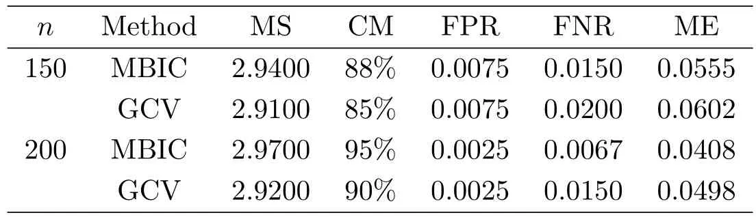
Table 1：Simulation results for model selection

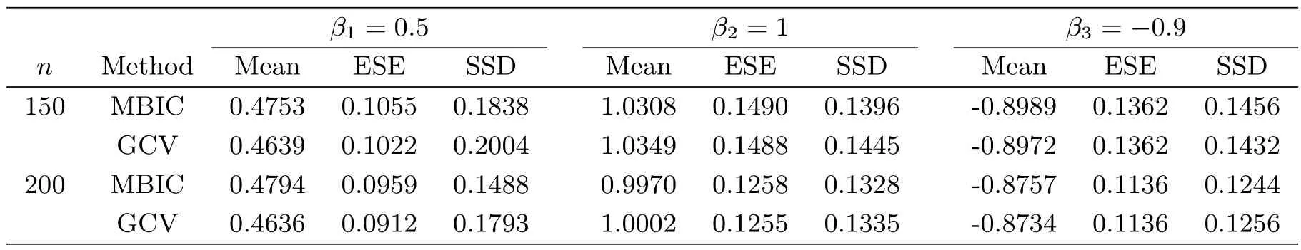
Table 2：Simulation results for parameter estimation

4 Concluding Remarks

Since the SICA penalty is modi fi ed from the transformedL1penaltypλ,τ(βj)=λ|βj|/(|βj| +τ)proposed by Nikolova[10],it is straightforward to extend the SPPL-MBIC method to the penalty function

whereλ(sparsity)andτ(concavity)are two positive tunning parameters,andfis an arbitrary function that satis fi es the following two hypotheses

(H1)f(x)is a continuous function w.r.tx,which has the fi rst and second derivative in[0,1];

(H2)f′(x)≥ 0 on the interval[0,1]and

It is noteworthy thatpλ,τ(βj)is the SELO penalty function proposed by Dicker et al.[5]when we takef(x)=log(x+1).

[1]Cai J,Fan J,Li R,Zhou H.Variable selection for multivariate failure time data[J].Biometrika,2005,92(2)：303-316.

[2]Chen X.Superlinear convergence of smoothing quasi-Newton methods for nonsmooth equations[J].J.Comput.Appl.Math.,1997,80(1)：105-126.

[3]Chen X.Smoothing methods for nonsmooth,nonconvex minimization[J].Math.Prog.,2012,134(1)：71-99.

[4]Cox D R.Regression models and life tables(with discussion)[J].J.Royal Stat.Soc.,1972,34(2)：187-220.

[5]Dicker L,Huang B,Lin X.Variable selection and estimation with the seamless-L0penalty[J].Stat.Sinica,2013,23：929-962.

[6]Fan J,Li R.Variable selection for Cox’s proportional hazards model and frailty model[J].Ann.Stat.,2002,30(1)：74-99.

[7]Fan J,Peng H.Nonconcave penalized likelihood with a diverging number of parameters[J].Ann.Stat.,2004,32(3)：928-961.

[8]Huang J,Liu L,Liu Y,Zhao X.Group selection in the Cox model with a diverging number of covariates[J].Stat.Sinica,2014,24：1787-1810.

[9]Lv J,Fan Y.A uni fi ed approach to model selection and sparse recovery using regularized least squares[J].Ann.Stat.,2009,37(6A)：3498-3528.

[10]Nikolova M.Local strong homogeneity of a regularized estimator[J].SIAM J.Appl.Math.,2000,61(2)：633-658.

[11]Nocedal J,Wright S.Numerical optimization(2nd ed.)[M].New York：Springer,2006.

[12]Shi Y Y,Cao Y X,Jiao Y L,Liu Y Y.SICA for Cox’s proportional hazards model with a diverging number of parameters[J].Acta Math.Appl.Sinica,English Ser.,2014,30(4)：887-902.

[13]Tibshirani R.The lasso method for variable selection in the Cox model[J].Stat.Med.,1997,16(4)：385-395.

[14]Wang H,Li B,Leng C.Shrinkage tuning parameter selection with a diverging number of parameters[J].J.Royal Stat.Soc.,Ser.B(Stat.Meth.),2009,71(3)：671-683.

[15]Wang H,Li R,Tsai C L.Tuning parameter selectors for the smoothly clipped absolute deviation method[J].Biometrika,2007,94(3)：553-568.

[16]Xu C.Applications of penalized likelihood methods for feature selection in statistical modeling[D].Vancouver：Univ.British Columbia,2012.

[17]Zou H,Hastie T,Tibshirani R.On the “degrees of freedom” of the lasso[J].Ann.Stat.,2007,35(5)：2173-2192.

发散维数SICA惩罚Cox回归模型的一种修正BIC调节参数选择器

石跃勇1,3,焦雨领2,严 良1,曹永秀2

(1.中国地质大学(武汉)经济管理学院,湖北武汉 430074)(2.中南财经政法大学统计与数学学院,湖北武汉 430073)(3.中国地质大学(武汉)资源环境经济研究中心,湖北武汉 430074)

本文研究了发散维数SICA惩罚Cox回归模型的调节参数选择问题,提出了一种修正的BIC调节参数选择器.在一定的正则条件下,证明了方法的模型选择相合性.数值结果表明提出的方法表现要优于GCV准则.

Cox模型;修正BIC;惩罚似然;SICA惩罚;光滑拟牛顿

O212.1

on：62N01;62N02

A Article ID：0255-7797(2017)04-0723-08

date：2016-11-10Accepted date：2016-12-20

Supported by National Natural Science Foundation of China(11501579);Fundamental Research Funds for the Central Universities,China University of Geosciences(Wuhan)(CUGW150809).

Biography：Shi Yueyong(1984-),male,born at Luzhou,Sichuan,lecturer,major in biostatistics.

Cao Yongxiu.