A Tree-Based Approach for Efficient and Accurate Conjunction Analysis

Michael Mercurioand Puneet Singla

A Tree-Based Approach for Efficient and Accurate Conjunction Analysis

Michael Mercurio1and Puneet Singla2

Conjunction analysis is the study of possible collisions between objects in space.Conventional conjunction analysis algorithms are geared towards computing the collision probability between any two resident space objects.Currently,there are few heuristic methods available to select which objects should be considered for a detailed collision analysis.A simple all-on-all collision analysis results in an O(N2)procedure,which quickly becomes intractable for large datasets.The main objective of this research work is to preemptively determine which catalogued objects should be considered for a more detailed conjunction analysis,significantly reducing the numberof object pairs to be investigated.The heart of the approach lies in the efficient kd-tree algorithm.It has been found that this binary search method significantly reduces computational cost to a tractable complexity of O(NlogN).The conventional tree-based search is modified slightly by accounting for probabilistic nearest neighbors via the Hellinger Distance.Finally,the method is extended to account for Non-Gaussian errors via the inclusion of Gaussian Mixture Models.It has been found that the reduced computational complexity of the kd-tree is maintained,while the applicability of the method is extended to uncertain cases.

1 Introduction

Space debris and Resident Space Objects(RSOs)are tracked and logged to monitor the significant threat they pose to current space operations.Currently,debris of approximately five centimeters can be tracked and logged,and from this,a catalog of over 21,000 objects currently in orbit is monitored and updated[Mercurio,Singla,and Patra(2012)].Additionally,the uncertainties present from measurement noise and errors greatly affect the accuracy of the catalog.A relatively small piece ofdebris can render a satellite useless,and create more debris.Hence,no single item should be barred from conjunction analysis.The examination of this risk,typically referred to as conjunction analysis,requires extensive computational effort due to the combinatorial nature of the algorithms,and the number of RSOs considered.The unintentional collision between Russia’s Cosmos 2251 satellite and a US Iridium satellite advocates a need for an accurate and efficient conjunction analysis algorithm[Mercurio,Singla,and Patra(2012)].

With the inherent uncertainties in the motion of the space objects,the collision is no longer just the intersection of the two trajectories.Rather,one has to consider the intersection of multiple realizations of orbit trajectories of both objects.This naturally leads to the notion of conjunction probability[Vallado(2001)].A thorough conjunction analysis requires a significant amount of information about the RSOs,including time of closest approach,relative distance,and probability of collision.The simplest form of the conjunction analysis begins with calculating the distance between the greatest perigee and the smallest apogee from the two RSO orbits.The collision of the two RSOs will be analyzed further if this distance is less than some specified tolerance.If the distance is less than the specified tolerance,an error ellipsoid is created about the first RSO of interest based on its covariance matrix.The ellipsoid is placed such that its major axis is aligned with the RSO’s velocity vector.From here,the probability of collision between the two RSOs is computed[Vallado(2001)].Computing the accurate conjunction probability is often difficult and hence many reasonable approximations are made to evaluate this probability leading to different computational methods[Akella and Alfriend(2000);Alfano(2007,2009);Carpenter(2004,2007);Carpenter,Markley,and Gold(2012);Cho,Chung,and Bang(2012);Milani,Chesley,Chodas,and Valsecchi(2002);Vallado(2001);Adurthi and Singla(2015)].

Although a great detail of attention has been paid to compute the collision probabilities between any single pair of RSOs, little attention has been paid to select a subset of catalogued objects,which has highest probability of collision.This generally requires an exhaustive search of catalogued objects.Of course,certain combinations are exempt,such as collisions between objects in low-Earth orbit(LEO)and objects in Geosynchronous orbit(GEO).A naive search would require all object-pairs to be considered for potential collision candidates.This would result in computing the probability of collision between each and every object in a set,which,for a set of N objects,results in an O(N2)operation.Due to the increasing size of the space object catalog,a methodology is sought to assist in reducing the number of RSO pairs to be considered for detailed conjunction analyses.This research presents a method for intelligent selection of these RSO pairs to be further investigated via more detailed conjunction analysis methods.While attempts have been made to reduce the computational overhead,these revised methods often require a form of space discretization,or a slightly reduced combinatorial analysis[Crassidis,S-ingla,McConky,and Sudit(2011);Mercurio,Singla,and Patra(2012)].It is these considerations that serve as the main motivation for this research.

Elementary nearest-neighbor searches involve computing the distance between all objects within a dataset,and determining the minimum distance values.Efficient sorting and storage algorithms can be introduced to assist in reducing the computational load associated with the nearest-neighbor search.Tree-based data structures,specifically kd-trees,are well-known for their efficient storage and retrieval properties[Bentley(1975)].Here,the dataset is conditioned about its median value,and the objects are recursively stored,and indexed,via nodes within the tree structure.The structure of the kd-tree lends itself to efficient determination of an objects nearest neighbors.The conventional application,however,is limited to deterministic datasets,i.e.the data is known perfectly.Thus,in order to apply the kd-tree to uncertain cases,some modifications must be made.

Deterministic nearest-neighbor algorithms rely on computing a distance value between object-pairs within a dataset. Some datasets, such as RSO locations, are characterized by probability density functions(PDFs)and thus,a deterministic nearestneighbor search is not directly applicable.Therefore,a probabilistic distance metric is required to determine the an object’s nearest neighbor in a probabilistic sense.These metrics measure the amount of shared area between two PDFs and thus,offer a value linked to the probability of collision.While some of these measures offer closed-form expressions for Gaussian uncertainties,direct extensions to Non-Gaussian cases often involve expensive numerical integration procedures.This can be circumvented by first approximating Non-Gaussian PDFs as a finite weighted sum of independent Gaussian kernels.From here,a novel approach to compute a probabilistic distance is investigated,relying on a linear programming framework.Preliminary investigations using this methodology are available in Refs.Mercurio,Singla,and Patra(2012,2013).However,the sum of these necessary modifications serves as the basis for this research work.

First,an introduction to kd-trees and nearest neighbor searches in detailed.Then,for uncertain RSO position,methods for characterizing uncertainty are discussed,followed by a brief overview of probabilistic distance metrics.Next,as accurate representations of uncertainty are sought,extending the computation of probabilistic distance metrics to GMMs is presented.Finally,a modified nearest neighbor algorithm is detailed,offering an extension of the conventional kd-tree to uncertain scenarios.Numerical results are provided to demonstrate the efficacy of the proposed approach.

2 Proposed Methodology

As discussed earlier,conventional conjunction analysis algorithms require combinatorial analyses,resulting in O(N2)operations.An approach is sought to reduce the computational burden,while maintaining accurate and verifiable results.In the framework of data storage and retrieval algorithms,the kd-tree structure is a wellknown methodology.When applied to a nearest neighbor search,the kd-tree offers an ideal computational load of O(NlogN),which is a significant reduction from the conventional conjunction analysis algorithms.

2.1 kd-Trees

Typical data structures,such as arrays,can be used for storage and searching of a dataset.In this case,there is no rule as to how the data is stored or indexed.Thus,the search and retrieval operation can be accelerated by the introduction of a better storage algorithm.It is this purpose that warrants the use of tree data structures.A tree is a hierarchical data structure created by efficiently organizing a dataset[Bentley(1975)].A tree structure contains nodes,which store information,or points,from the dataset.Each node may have descendants,or children,which store points related to the parent node.This organization lends itself to rapid searching and recovery of data within the tree.While numerous trees exist for data storage,kd-trees and octrees are the most prominent for three-dimensional datasets.

Octrees are tree data structures in which each node possesses a maximum of eight descendants[Sundar and Sampath(2007)].In dividing the domain of interest,cubes(octants)are created and further divided until each datapoint lies in its own octant.Octrees create a physical mesh,and are typically used for collision analysis of solid objects,and finite element analysis.As opposed to octrees,kd-trees are data structures in which each node has a maximum of two descendants.These data structures are favored due to their low computational and storage requirements,as no physical mesh is created.An example kd-tree of dimension two is depicted in Fig.1.

For this analysis,a kd-tree implementation was chosen over an octree as a physical mesh need not be created.The nodes of a kd-tree are not physically created;they are used simply to index the points in a given dataset.In general,the kd-tree implementation is described as“top-down”as this is the direction of construction of the tree[Press(2007)].The root box,which can be described as the space surrounding the entire dataset,is first initialized.The root box is then divided along a specified dimension,typically the longest available,creating two nodes.Once divided,the location of each data point is examined to determine their respective placement in the kd-tree-if the item is leftward of the division,it is placed into the leftmost n-ode,and vice versa for a rightward item.From here,the procedure is repeated until only one item lies in each node(box).Upon completion of the final divisions,the remaining boxes,each populated with one or two data points,are termed leaves.This insertion procedure is termed recursion,and its simplicity governs the favored implementation of kd-trees.Although the original order of the dataset is stored elsewhere,the dataset is organized in increasing order during construction of the kd-tree.A simplified kd-tree algorithm is presented as Alg.1[Press(2007)].An schematic detailing an example application of this algorithm is depicted in Fig.2.

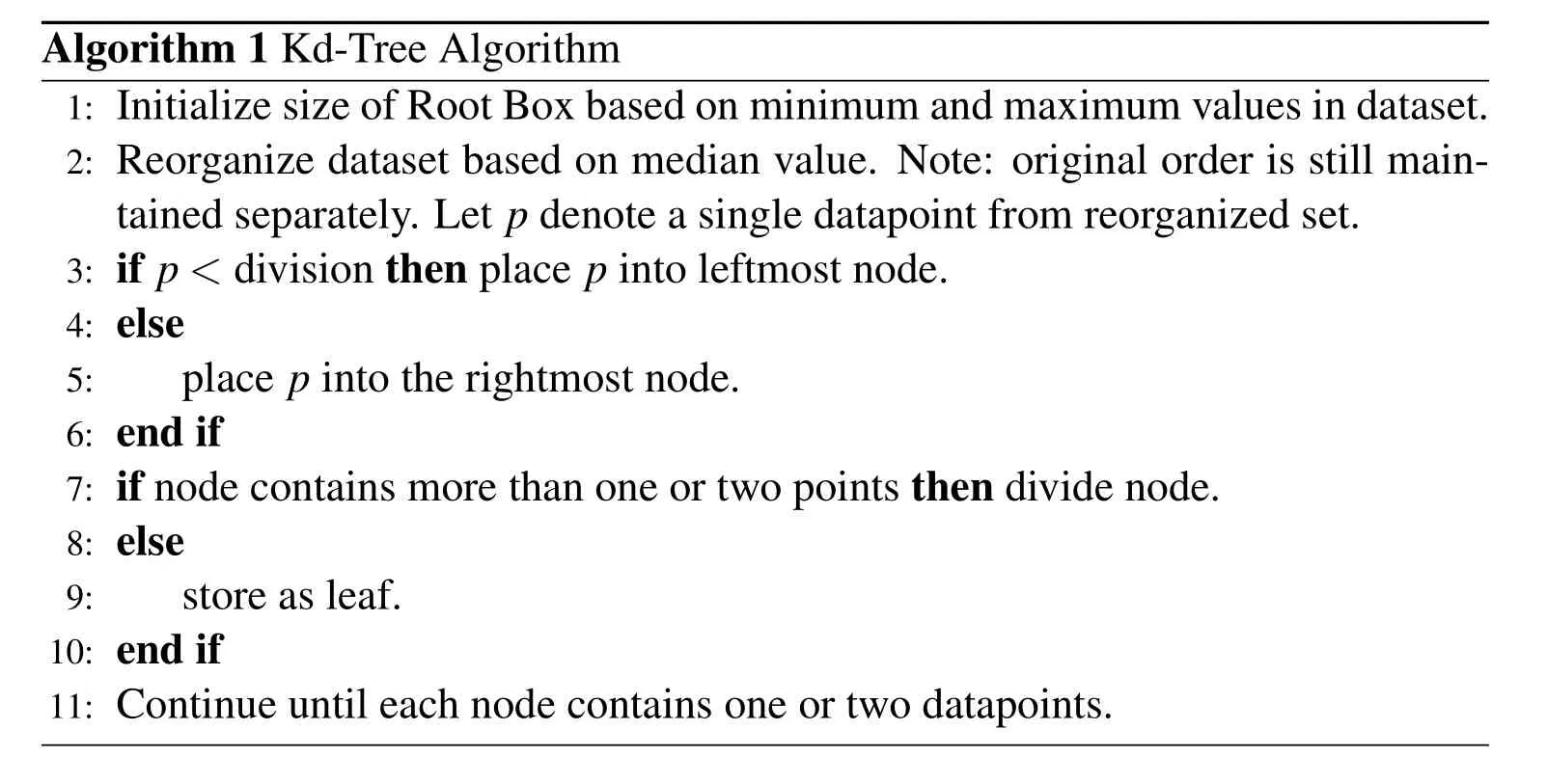
Algorithm 1 Kd-Tree Algorithm 1:Initialize size of Root Box based on minimum and maximum values in dataset.2:Reorganize dataset based on median value.Note:original order is still maintained separately.Let p denote a single datapoint from reorganized set.3:if p＜division then place p into leftmost node.4:else 5: place p into the rightmost node.6:end if 7:if node contains more than one or two points then divide node.8:else 9: store as leaf.10:end if 11:Continue until each node contains one or two datapoints.

Figure 1:Example kd-tree of Dimension Two

Tree data structures are well known for their computational efficiency in obtaining accurate and verifiable results.As the kd-tree is defined based on recursive principles,the workload can be scaled by clever programming principles.The kd-tree construction discussed above can be analyzed to determine the cost required.

Figure 2:Example Construction of kd-tree of Dimension Two

2.1.1 Computational Cost of kd-Tree Construction

The most expensive portion of creating the kd-tree is the insertion algorithm.By inserting points into a tree one by one,the best possible computational load is O(N)[Moore and Hall(1990)].This cost is reduced by utilizing a balanced kdtree,which ensures that the domain is divided such that an approximately equal number of points lie on each side of each division[Press(2007)].One method of ensuring a balanced kd-tree is to divide the domain along the longest dimension at each step[Moore and Hall(1990)].By dividing the domain of interest as such,and preconditioning the dataset about the median value,a recursive insertion algorithm can be used to scale the insertion algorithm to O(NlogN).The recursion principle scales the computational cost to[Wald and Havran(2006)]:

Where T(N)is the operational time for N items.Eq.1 is valid for N≥2.ForN=1,the cost is simply T(1)=1,as only one item is stored.The multiplicative factor of 2 is applied as the domain is halved at each iteration,creating two subdomains.Further,the number of items to be considered is also halved,resulting in a cost of T(N/2)at the current iteration,e.g.each subdomain contains approximately N/2 items.Finally,the N term is present as the cost to find the median of the dataset.It must be noted that this is an approximation of the computational cost for any dimensionality,as the dimension of the dataset simply scales the cost by a constant.Substituting the recurrence relations yields:

From Eq.4,it can be seen that after three iterations,the following relationship can be inferred:

This is the cost required after p applications of the recursive algorithm to reduce the dataset to a single item from N initial items.The value of p can be determined as N=2p→p=log2N.Thus,the total cost for N items is:

The final equality follows from the fact that as N is increased,Nlog2N will overtake N.Additionally,the base of the logarithm is not included,as the base can be changed via a constant multiplier,which is absorbed in the“big-O”notation.Eq.7 provides the cost of constructing the kd-tree for a conditioned dataset.However,as noted above,the preconditioning step requires sorting the dataset in regards to the median value,a O(k·NlogN)operation.Thus,the total computational load to construct the kd-tree is O(NlogN)+O(k·NlogN),which is simply O(NlogN)in“big-O”notation.

2.2 Conventional Deterministic Nearest Neighbor Search

The data storage structure of kd-trees can be exploited to obtain information about the dataset with increased efficiency.As the dataset is preconditioned based on increasing values of object locations,objects surrounding a specific datapoint can be readily retrieved[Moore and Hall(1990);Press(2007)].

Kd-trees aid in NN searches by reducing the computational load required.The computational complexity of a conventional brute-force NN search isO(N2)whereas a kd-tree based search reduces this load to O(NlogN)on average,where N is the number of items considered[Bentley(1975)].It must be noted,however,that this is an average complexity.If the dataset is poorly conditioned,e.g.a sparse dataset,resulting in multiple empty nodes within the tree,the number of nodes investigated increases[Moore and Hall(1990)].A kd-tree NN search algorithm is outlined as Alg.2[Press(2007)].An example application of this algorithm is depicted in Fig.3.This approach is carried-out using the example kd-tree from Fig.2.

2.2.1 Computational Cost of Conventional Deterministic Nearest Neighbor Search The algorithm complexity can be determined by analyzing the number of possible operations for each iteration of the algorithm.Initially,there are N possible operations,as any object is a candidate nearest neighbor.For the second iteration,the algorithm has eliminated objects on the current side of the domain.This reduces the number of potential operations to N/2,as the balanced kd-tree assures an approximately equal number of objects on either side of each division.The third iteration splits the current side of the domain once again,reducing the number of possible operations to N/4.This trend continues until,at worst,the final iteration leaves a single object to investigate.Tab.1 depicts this trend.An example schematic of the algorithm complexity analysis is shown in Fig.4 using seven items in a balanced kd-tree.This again shows the reduction in possible operations at each iteration,where the hatched regions are eliminated at the start of the given iteration.It can be seen that for the pthiteration,the resulting number of possible operations is O(N/2k).It is also known that the last iteration has but one iteration,i.e.the final iteration number is the iteration that corresponds to the algorithm investigating a single point.Therefore,the number of iterations can be computed as

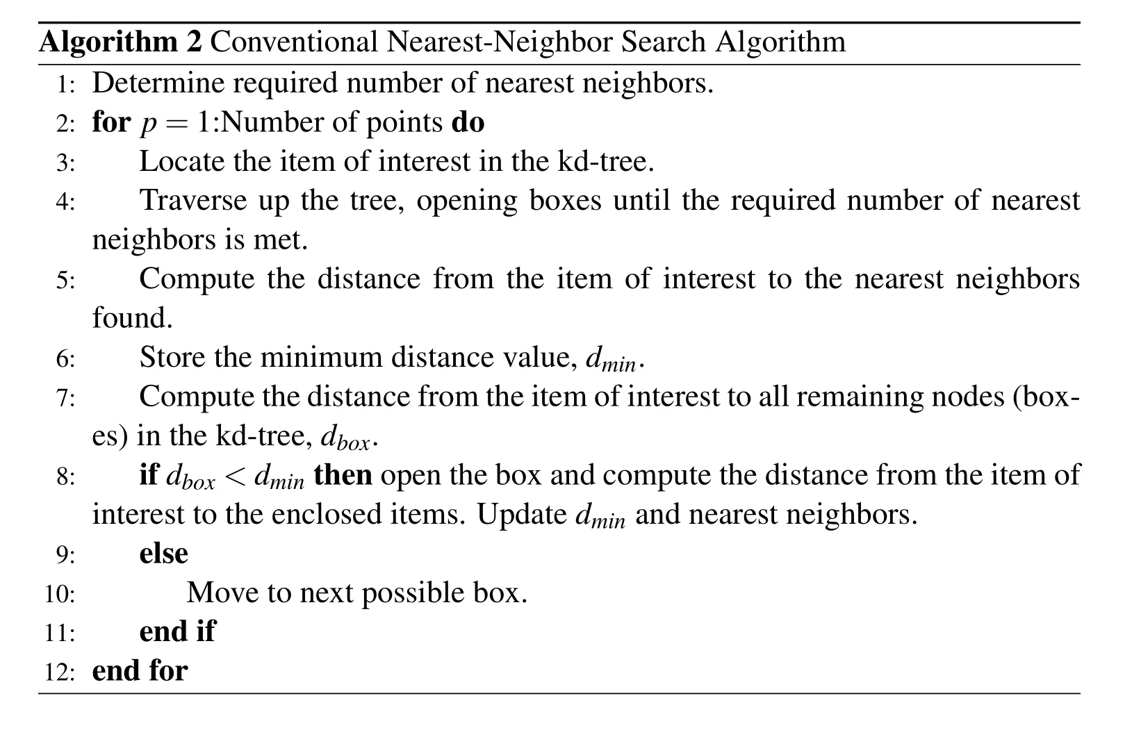
Algorithm 2 Conventional Nearest-Neighbor Search Algorithm 1:Determine required number of nearest neighbors.2:for p=1:Number of points do 3: Locate the item of interest in the kd-tree.4: Traverse up the tree,opening boxes until the required number of nearest neighbors is met.5: Compute the distance from the item of interest to the nearest neighbors found.6: Store the minimum distance value,dmin.7: Compute the distance from the item of interest to all remaining nodes(boxes)in the kd-tree,dbox.8: if dbox＜dminthen open the box and compute the distance from the item of interest to the enclosed items.Update dminand nearest neighbors.9: else 10: Move to next possible box.11: end if 12:end for

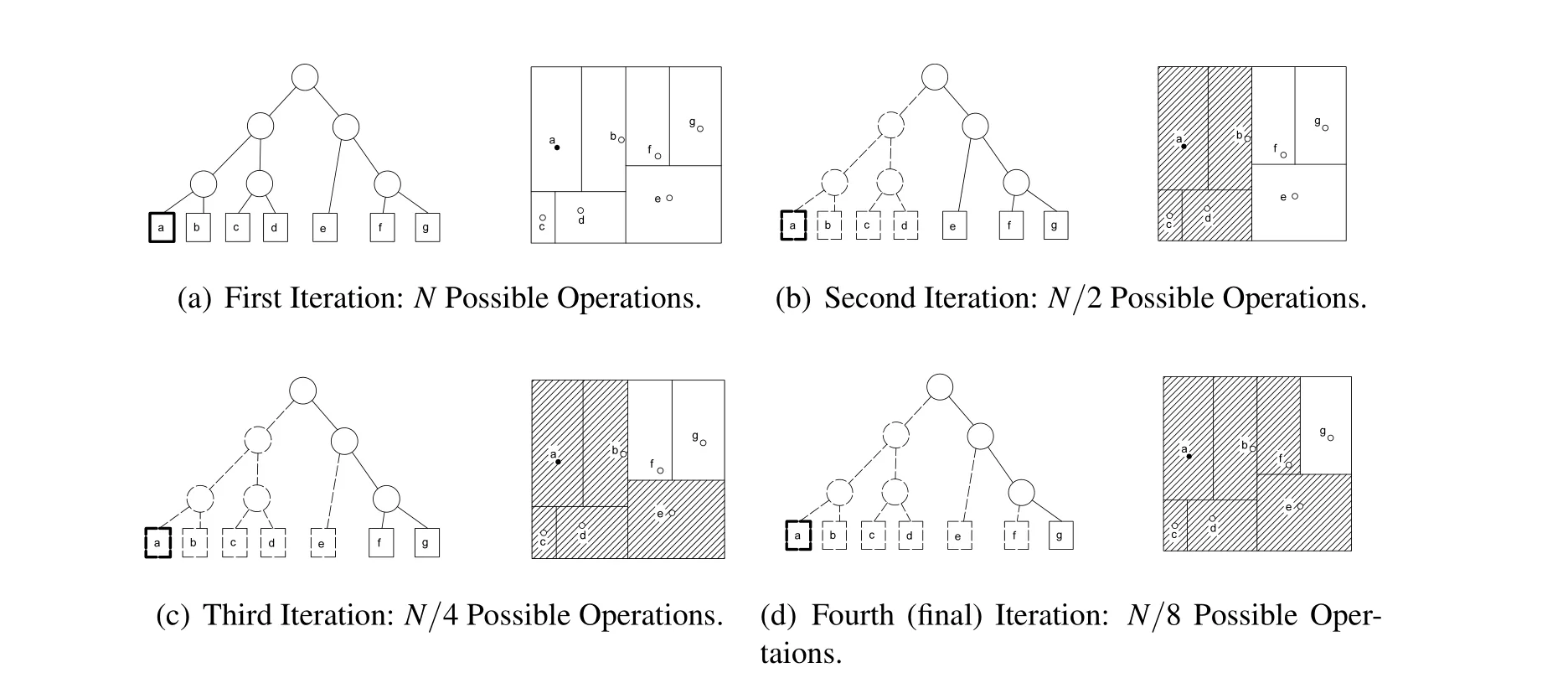
Figure 4:Example Algorithm Complexity Analysis

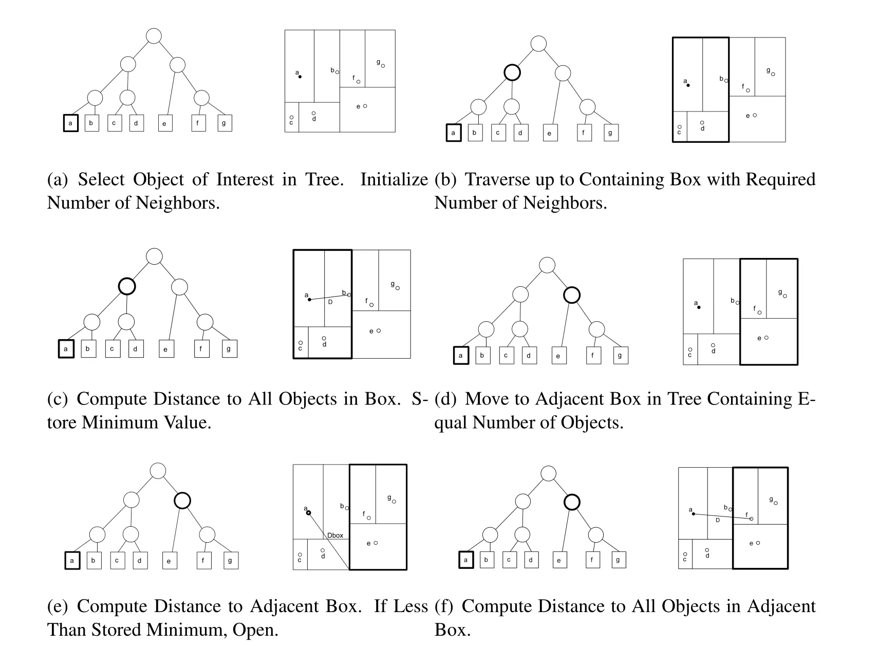
Figure 3:Example Nearest Neighbor Search

From Eq.8,it can be seen that the computational complexity of the nearest neighbor search algorithm is O(logN)for a single object’s nearest neighbor.For all N objects,the complexity scales to O(NlogN).Note that the base of the logarithm is not specified,as log bases can be changed via a constant,which is ignored in“big-O”notation[Cormen,Leiserson,Rivest,and Stein(2001)].It must be noted that this complexity only accounts for the nearest-neighbor search.The total complexity,including constructing the kd-tree would be O(NlogN)+O(NlogN),which is,of course,O(NlogN)in“big-O”notation.

The conventional NN search via a kd-tree implementation is clearly more efficient than a brute-force NN search algorithm,which requires the computation of the distance between all possible combinations of items.It can immediately be seen that the kd-tree lends itself towards conjunction analysis,however,the conventional implementation cannot directly account for uncertain RSO locations.Here,a probabilistic distance metric is required

Table 1:Possible Operations

2.3 Overview of Probabilistic Distance Metrics

As seen in Alg.2,the conventional nearest neighbor search requires a comparison of distance values between two RSOs.For the case of uncertain RSO positions,the Euclidean distance metric does not offer insight towards the likelihood of collision between any two objects.The standard approach to computing the collision probability relies on integrating the overlapping region between two PDFs[Mercurio,Singla,and Patra(2012,2013)].This approach,however,yields a value of probability and thus,cannot be employed as a distance metric.It is therefore appropriate to find a proper metric to represent the probability of collision between two RSOs.For this research,the Kullback-Leibler divergence,the Bhattacharyya Distance,and the Hellinger Distance have been considered.

The probabilistic metrics described possess closed-form solutions for cases in which all uncertainties are characterized by Gaussian distributions.Uncertainties characterized by non-Gaussian distributions,however,must be treated via numerical integration procedures.For the case of two mixture models,however,a simplified approach exists.

2.4 Probabilistic Distance Metrics for Mixture Models

The lack of closed-form expressions for distance metrics in the presence non- Gaussian uncertainties limits their applicability to non-efficient algorithms. Numerical integration methods can be used to evaluate these distances,however,these procedures are often computationally expensive[Mercurio,Singla,and Patra(2013)].Instead,a method is sought to exploit the formulation of GMM distributions,and avoid expensive numerical integration procedures.

Recent research in uncertainty characterization has focused on fusing accurate PDF representations with computationally efficient methods. Recently, different variants of Gaussian Mixture Models(GMM)have found special interest in the field of orbital mechanics for uncertainty propagation[Horwood,Aragon,and Poore(2011);Vishwajeet,Singla,and Jah(2014);Vishwajeet and Singla(2014)],orbit determination[DeMars and Jah(2013)],and conjunction assessment[Vittaldev and Russell(2013);Mercurio,Singla,and Patra(2013)].All GMM based algorithms are based upon the assumption that the probability density function of the state can be approximated by a mixture of Gaussian kernels[Terejanu,Singla,Singh,and Scott(2008,2011)].The mean and covariance information for each Gaussian kernel is computed independently.Different algorithms incorporate various criteria and corresponding rationale for selection of the Gaussian kernels and the computation of weight of each Gaussian kernel.

These methods are often a trade-off between expensive,but highly-accurate,Monte Carlo methods,and efficient,but ultimately inaccurate,Gaussian-based methods.Due to the nature of the GMM formulation,however,many properties of Gaussian PDFs can be exploited[DeMars,Cheng,and Jah(2014);Mercurio,Singla,and Patra(2013)].

Where µ,and Σ represent the mean vector and covariance matrix,respectively.In short-hand notation,the Gaussian density with mean µ and covariance Σ can be expressed as N(x x x|µ,Σ).An n-dimensional GMM is simply a weighted sum of ndimensional Gaussian density functions,expressed as[Mercurio,Singla,and Patra(2013)]:

Where wiis the weight of the ithGaussian component.The weights are subject to the constraint:

GMMs can be used to represent non-Gaussian uncertainties and thus,offer additional accuracy in computing collision probabilities.As GMMs are comprised of a weighted-sum of Gaussian components,many formulae developed for Gaussian uncertainties can be extended simply.

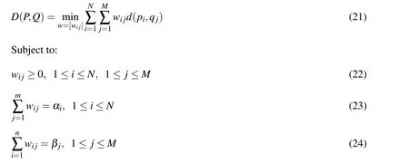
Where,as above, αiand βjare the weights of the mixture model components,piand qjare any chosen probability density functions(components of mixture models P and Q,respectively),wijis the weight of the ijthdistance component,and d(pi,qj)is the probabilistic distance metric of choice between the ithand jthcomponents of the chosen mixture models.The optimized distance will satisfy the same properties as the metric chosen for inter-component distances,e.g.if d(pi,qj)satisfies the non-negativity and symmetry properties,then D(P,Q)will also satisfy these properties[Liu and Huang(2000)].This distance computation may be used with any probabilistic distance metric, however, the Hellinger Distance will be employed due to the fact that it is a proper metric.The optimization problem can thus be posed as:

The linear programming(LP)problem defined above is convex,as the objective function and equality constraints are linear.Therefore,if an optimum solution can be found,global optimality is guaranteed[Arora(2004)].Additionally,the LP problem possesses the following qualities:(1)the following trivial,feasible,non-optimal solution exists,which satisfies the constraints:wij= αiβj(the linear programming problem is therefore feasible), and (2) the objective function is upperbounded(by unity when the Hellinger Distance is used).

2.5 Modified Probabilistic Nearest Neighbor Search

The conventional nearest-neighbor search relies on deterministic locations of RSOs.For uncertain locations,however,a modified approach must be derived.The main challenge lies in computing the distance-to-box,dboxto identify the appropriate tree node or box containing the nearest neighbor.Many modifications were considered involving various methods of modifying the distance-to-box function in the nearest-neighbor algorithm. The first of these approaches required the Hellinger distance for inter-RSO analyses,while the Euclidean distance was maintained for the distance-to-box[Mercurio,Singla,and Patra(2012,2013)].This resulted in comparing the Hellinger distance with the Euclidean distance prior to investigating RSOs within a given box,as shown in Fig.5.As the Hellinger distance is normalized,the values obtained will almost always be less than those obtained via the Euclidean distance in a non-normalized space.Additionally,use of a normalized space is not advisable,as the values obtained from two different distance metrics would be compared.Thus,this approach did not yield accurate results,and a new approach was sought based on the probabilistic nature of the problem.Another approach involved representing a given box as a joint Gaussian PDF comprised of the contained RSOs,as shown in Fig.6.This approach failed to yield accurate results as the covariance of the joint PDF is weighted by the inverse of the sum of the component covariances.Therefore,for large covariances,the resulting joint PDF possesses a small covariance.Therefore,in all cases considered,no overlap would occur and thus,the Hellinger distance would assume a value of unity,and the contained RSOs would not be investigated further.The final approach consisted of approximating a given box as a uniform density function,as shown in Fig.7.As with the previous methods,this approach fails to capture uncertainties extending beyond the limits of the containing box.Therefore,if no overlap is present between the PDF of the current RSO and the box of interest,the RSOs contained will not be investigated.Finally,a modification to the algorithm described in Alg.3 is considered.First,the kd-tree is formed based upon the mean locations of the RSOs.Regarding the interactions between RSOs,the Hellinger distance is employed to obtain a “distance”value inversely proportional to the overlap of the PDFs and thus,the probability of collision.In addition to this metric,the Euclidean Distance is computed between RSOs.This serves as comparison values for the distance-to-box computation.It is noted that the structure of the nearest-neighbor search algorithm is maintained.The modified algorithm is described as Alg.3.

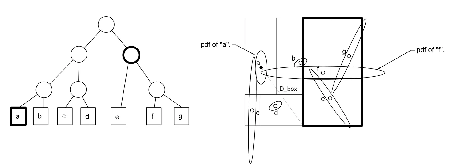
Figure 5:Distance-to-Box-Euclidean Distance Method

Figure 6:Distance-to-Box-Joint Gaussian Method

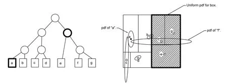
Figure 7:Distance-to-Box-Uniform Distribution Method

?

Comparing Alg.3 with Alg.2,it can be seen that the modified nearest neighbor algorithm is of the same computational complexity.While,at each iteration,the number of possible operations is increased by a factor of two,due to the inclusion of the Euclidean distance metric,the computational complexities differ only by a constant,which is ignored in “big-O”notation.With the proposed approach detailed,numerical test cases are presented next.

3 Numerical Results

This section provides numerical results to demonstrate the efficacy of the proposed approach.All simulations were run on a 2.3 GHz Intel Core i7 machine,with 4 GB of RAM,and all code written in C++.To perform comparisons,sets of 200,2,000,5,000,and 10,000 RSOs have been pseudo-randomly generated in LEO orbits.

First,a scenario is examined where position uncertainties in each RSO are governed by Gaussian probability density functions.Each RSO assumed to possess a diagonal covariance matrix,with variances between 100 and 10,000 km.The large variance values are chosen to ensure interaction between the RSOs.A second scenario will quantify the uncertainty associated with each RSO as a GMM containing six components with equal weights.The mean of each Gaussian component(χi)is generated by:

Tab.2-Tab.5 list the top 10 candidates for collision in the case of Gaussian position errors while Tab.6-Tab.9 list top 10 candidates for collision in the case of non-Gaussian position errors.The result from the proposed kd-tree based approach are compared with the brute force(i.e.exhaustive search)way of identifying the top 10 collision candidates.As expected the proposed method accurately captures the top ten nearest-neighbors for RSOs with both the Gaussian position errors and GMM position errors.Furthermore,Fig.8 shows the CPU time required for all the methods and Fig.9 shows the number of comparisons required by each approach.From these figures,it can be seen that the proposed method significantly outperforms brute-force methods,and follows the O(NlogN)trend as expected.Additionally,the number of iterations required for Gaussian uncertainties is equivalent to that of the GMM uncertainties.Due to the optimization routines required,the CPU time for the GMM case is somewhat greater than that of Gaussian errors.The number of iterations required,however,is approximately equal for both cases.Additionally,Tab.8 shows only the time required to carry out the nearest-neighbor searches.Eq.10 shows the time required to create the kd-tree for all cases investigated.This value includes the CPU time required to sort the dataset,and construct the kd-tree.It can be seen that the tree creation does not add a significant amount of time to the total time required to carry out the proposed methodology.Additionally,accounting for the time to create the kd-tree,the proposed methodology still offers a significant improvement over the brute-force counterpart.

Next,the nearest neighbor to each RSO is computed by making use of the proposed approach and compared against the brute force method(i.e.exhaustive search).Tab.11 lists the percentage accuracy in identifying the nearest neighbor as compared to the brute force method.From these results,it can be seen that at worst,the proposed method captures 98.6%of the nearest neighbors.Note that for the cases investigated,the level of accuracy is not necessarily the same between Gaussian and GMM uncertainties,as although the initial datasets are equivalent in each case,the GMM PDFs are generated using only the mean and covariance values the Gaussian PDFs.This results in a different set of PDFs and thus,the nearest neighbors may not coincide between both scenarios.However,this level of accuracy is expected,due to the assumptions made in formulating the proposed approach.By employing a deterministic distance metric in the distance-to-box function,the uncertain location of each RSO is not taken into account.Thus,an assumption is made,where only the mean values of the RSO locations are considered when deciding whether or not to investigate RSOs located in nodes far away from the current RSO.Thus,a probabilistic nearest neighbor may lie in a node far away from the current RSO,but in a deterministic sense,the algorithm avoids investigating that node.As discussed in Section 2.6,accounting for uncertain RSO locations when employing the distance-to-box function is an area of active research.

Finally,as the proposed method does not capture all of the nearest neighbors for a given scenario,a short failure analysis is carried out.Here,the 10,000 RSO cases are analyzed to ascertain,which nearest neighbors are “missed”.Tab.12 depicts the minimum Hellinger Distance values for the missed RSO encounters for both Gaussian and GMM uncertainties.It can be seen that although the proposed method captures a significant number of RSO pairs,it does miss an object-pair with a fairly low Hellinger Distance value,resulting in a moderately high probability of collision.Again,the level of inaccuracy is expected due to the deterministic distance-to-box function.

Table 2:Top 10 Results-Gaussian Uncertainties-200 RSOs.

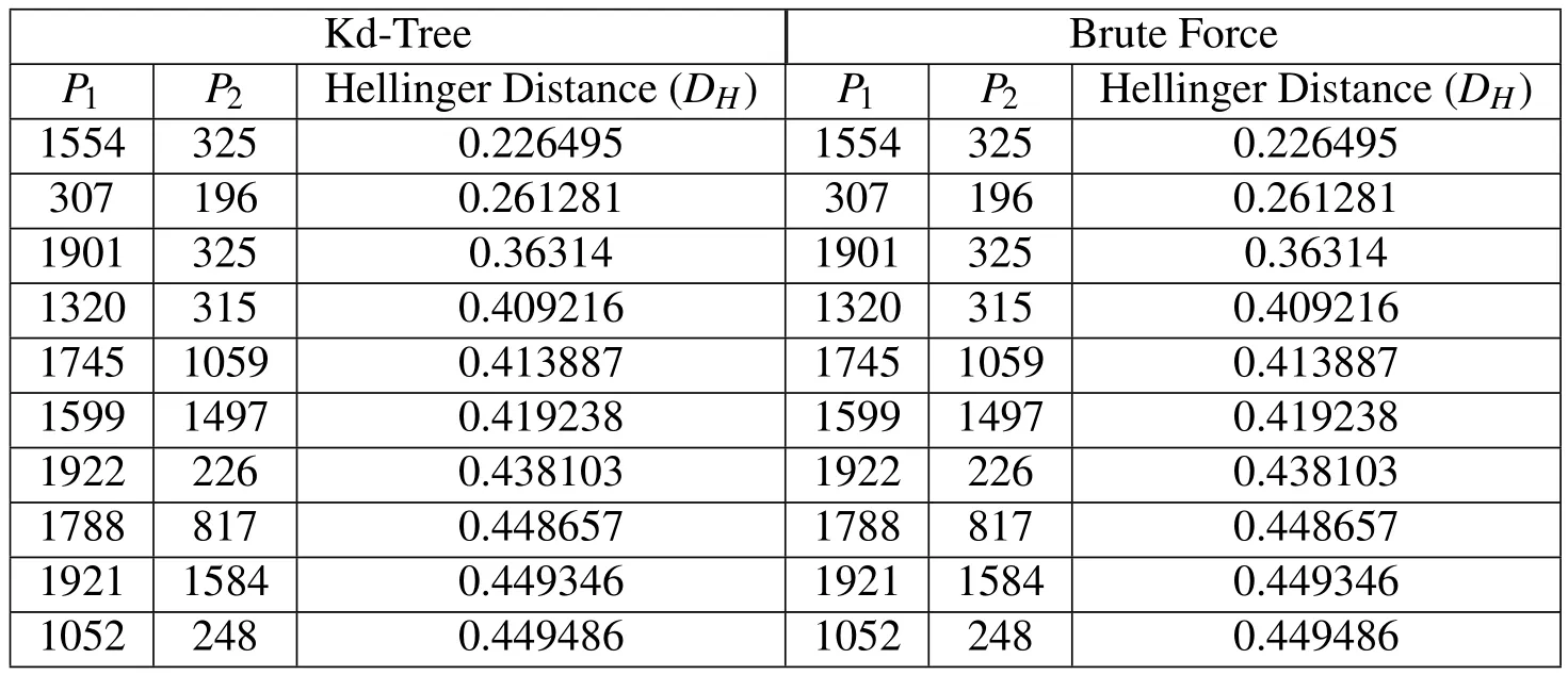
Table 3:Top 10 Results-Gaussian Uncertainties-2,000 RSOs.

Table 4:Top 10 Results-Gaussian Uncertainties-5,000 RSOs.

Table 5:Top 10 Results-Gaussian Uncertainties-10,000 RSOs.

Table 6:Top 10 Results-GMM Uncertainties-200 RSOs.

Table 7:Top 10 Results-GMM Uncertainties-2,000 RSOs.

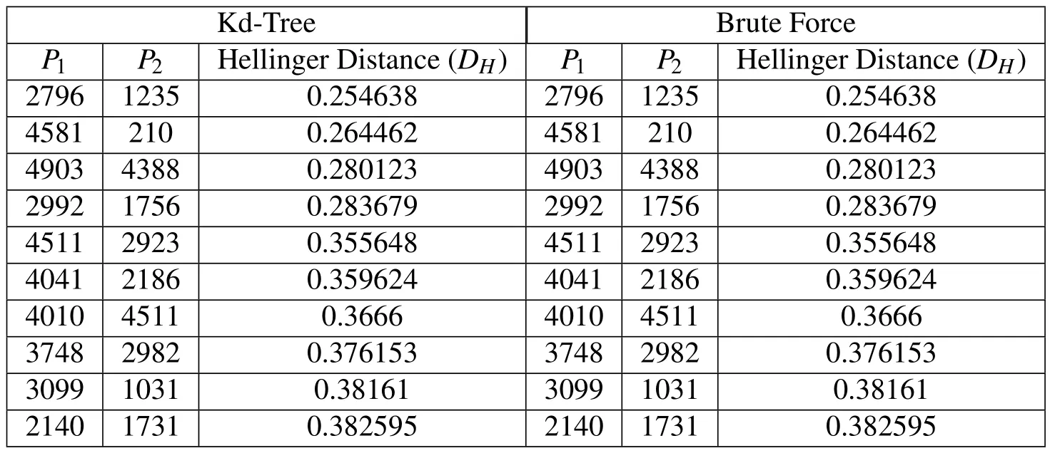
Table 8:Top 10 Results-GMM Uncertainties-5,000 RSOs.

Table 9:Top 10 Results-GMM-10,000 RSOs.

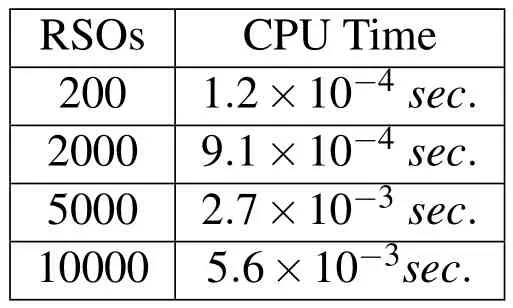
Table 10:CPU Time Required for Tree Creation.

Table 11:Percent of Nearest Neighbors Captured.

Table 12:Failure Analysis-10,000 RSOs.

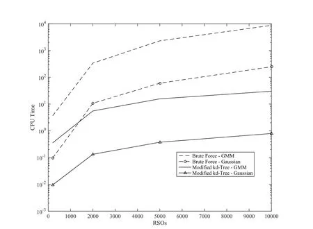
Figure 8:CPU Time Required for All Methods

4 Conclusions

Tree-based nearest neighbor searches are widely used for large datasets, as the number of computations is significantly reduced when compared to those required by a brute-force algorithm.Upon selecting the kd-tree due to its low-complexity,meshfree application,a modification was required in order to account for probabilistic nearest neighbors.For this,the Hellinger distance was chosen,as all properties of a distance metric are satisfied.Finally,to better quantify the uncertainties in RSO positions,each RSO position uncertainty is assumed to be represented by a Gaussian Mixture Model(GMM).With the necessary modifications made,the proposed method was implemented to obtain verifiable results against brute-force tests.

In the cases considered,the modified kd-tree method corroborated the most significant results obtained by brute-force methods,ensuring that the Hellinger dis-tance provides a link to the actual probability of collision and thus,the probabilistic nearest-neighbor.This research thus proposes a novel continuation of conjunction analysis algorithms.The modified kd-tree approach offers a significant improvement over conventional conjunction analysis algorithms,offering extreme reductions in required CPU time and iterations required.Further,Gaussian mixture models(GMMs)better quantify uncertainties when compared to standard Gaussian models,thus extending the applicability of the proposed method to scenarios with non-Gaussian errors.Finally,due to the linear programming-based distance metric computation,the inclusion of GMM uncertainties does not significantly increase the computational load required when compared to a conventional kd-tree approach.

It should be noted that the proposed approach is currently implemented for a single time instant.Propagation of RSO uncertainties will require some modification to the current algorithm,which is an area of active research.Although almost negligible at a single time instant,the time required to construct the kd-tree may pose a constraint to how often the tree should be constructed and thus,how often the nearest-neighbor search should be performed.However,it is anticipated that this methodology will offer insight towards accurate and efficient conjunction analy-sis for any encounter scenario by removing restrictive assumptions for the sake of computational efficiency.

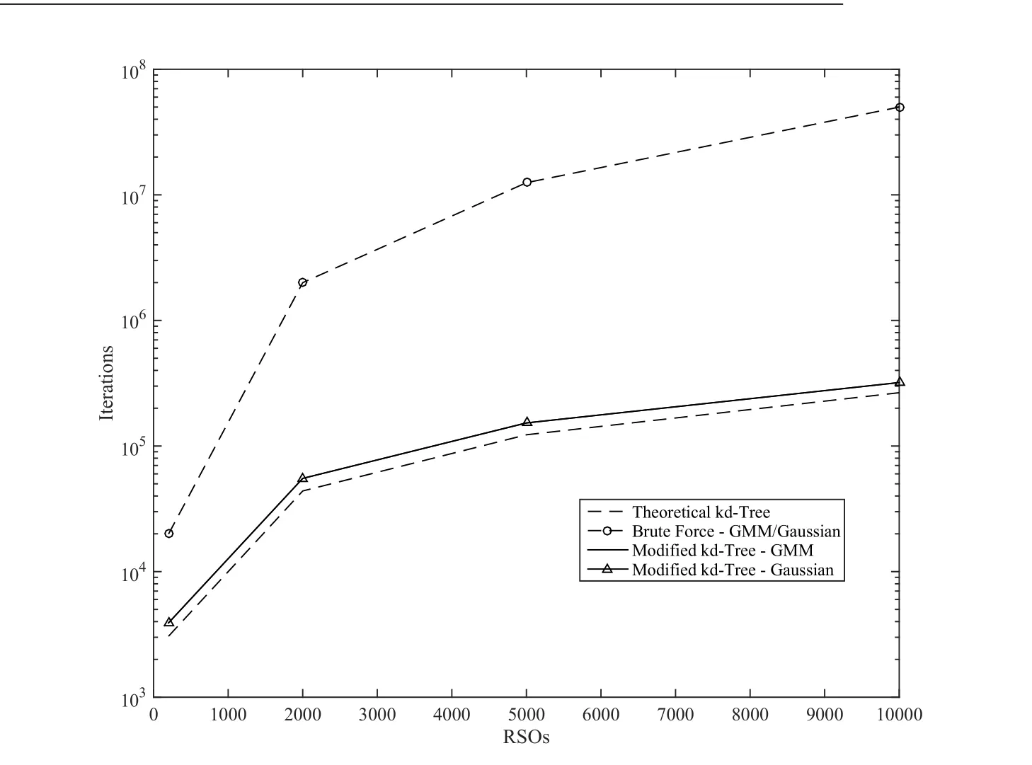
Figure 9:Iterations Required for All Methods

Acknowledgement:This material is based upon work supported by AFOSR grant FA9550-15-1-0313.

Adurthi,N.;Singla,P.(2015): Conjugate unscented transformation-based approach for accurate conjunction analysis.Journal of Guidance,Control,and Dynamics,pp.1–17.

Akella,M.R.;Alfriend,K.T.(2000):Probability of Collision Between Space Objects.Journal of Guidance,Control,and Dynamics,vol.23,no.5,pp.769–772.Alfano,S.(2007): Review of conjunction probability methods for short-term encounters.AAS Specialist Conference,Sedona,AZ.,Paper.

Alfano,S.(2009):Satellite Conjunction Monte Carlo Analysis.AAS Spaceflight Mechanics Mtg,Pittsburgh,PA.,Paper.

Arora,J.(2004):Introduction to optimum design.Academic Press.

Bentley,J.L.(1975):Multidimensional binary search trees used for associative searching.Communications of the ACM,vol.18,no.9,pp.509–517.

Carpenter,J.R.(2004):Conservative analytical collision probability for design of orbital formations.

Carpenter,J.R.(2007): Non-parametric collision probability for low-velocity encounters.Advances in the Astronautical Sciences.

Carpenter,J.R.;Markley,F.L.;Gold,D.(2012):Sequential probability ratio test for collision avoidance maneuver decisions.The Journal of the Astronautical Sciences,vol.59,no.1-2,pp.267–280.

Cho,D.-H.;Chung,Y.;Bang,H.(2012):Trajectory correction maneuver design using an improved B-plane targeting method.Acta Astronautica,vol.72,pp.47–61.

Cormen,T.H.;Leiserson,C.E.;Rivest,R.L.;Stein,C.(2001):Introduction to Algorithms.The MIT Press,2 edition.

Crassidis,J.;Singla,P.;McConky,K.;Sudit,M.(2011): Space Collision Avoidance.,no.October.

DeMars,K.J.;Cheng,Y.;Jah,M.K.(2014):Collision Probability with Gaussian Mixture Orbit Uncertainty.Journal of Guidance,Control,and Dynamics,vol.37,no.3,pp.979–985.

DeMars,K.J.;Jah,M.K.(2013):Probabilistic initial orbit determination using gaussian mixture models.Journal of Guidance,Control,and Dynamics,vol.36,no.5,pp.1324–1335.

Harsha,P.(2008):Lecture Notes:The Hellinger Distance,2008.

Horwood,J.T.;Aragon,N.D.;Poore,A.B.(2011): Gaussian sum filters for space surveillance:theory and simulations.Journal of Guidance,Control,and Dynamics,vol.34,no.6,pp.1839–1851.

Johnson,D.;Sinanovic,S.(2001):Symmetrizing the kullback-leibler distance.

Liu,Z.;Huang,Q.(2000):A new distance measure for probability distribution function of mixture type.Acoustics,Speech,and Signal Processing,2000.ICASSP’00.Proceedings,,no.2,pp.3–6.

Mercurio,M.;Singla,P.;Patra,A.(2012): A Hierarchical Tree Code Based Approach for Efficient Conjunction Analysis.AIAA/AAS Astrodynamics Specialist Conference.

Mercurio,M.;Singla,P.;Patra,A.(2013):A Non-Combinatorial Approach for Efficient Conjunction Analysis.InAAS/AIAA Astrodynamics Specialist Conference.

Milani,A.;Chesley,S.;Chodas,P.;Valsecchi,G.(2002): Asteroid close approaches:analysis and potential impact detection.Asteroids III,pp.55–69.

Moore,A.;Hall,T.(1990):Efficient memory-based learning for robot control.

Press,W.(2007):Numerical Recipes 3rd Edition:The Art of Scientific Computing,volume 3.Cambridge University Press.

Saul,L.(2011):CS291 Assignment 1,2011.

Sundar,H.;Sampath,R.(2007): Low-constant parallel algorithms for finite element simulations using linear octrees.Proceedings of the....

Terejanu,G.;Singla,P.;Singh,T.;Scott,P.(2008):Uncertainty propagation for nonlinear dynamic systems using Gaussian mixture models.Journal of Guidance,Control,....

Terejanu,G.;Singla,P.;Singh,T.;Scott,P.D.(2011): Adaptive Gaussian Sum Filter for Nonlinear Bayesian Estimation.IEEE Transactions on Automatic Control,vol.56,no.9,pp.2151–2156,DOI:10.1109/TAC.2011.2141550.

Vallado,D.(2001):Fundamentals of astrodynamics and applications.Springer.Vishwajeet,K.;Singla,P.(2014): Adaptive splitting technique for gaussian mixture models to solve kolmogorov equation.InAmerican Control Conference(ACC),2014,pp.5186–5191.IEEE.

Vishwajeet,K.;Singla,P.;Jah,M.(2014): Nonlinear uncertainty propagation for perturbed two-body orbits.AIAA Journal of Guidance,Control and Dynamics,,no.In-Press.

Vittaldev,V.;Russell,R.P.(2013):Collision probability for space objects using gaussian mixture models.InProceedings of the 23rd AAS/AIAA Space Flight Mechanics Meeting,volume 148.Advances in the Astronautical Sciences,Univelt San Diego,CA.

Wald,I.;Havran,V.(2006): On building fast kd-trees for ray tracing,and on doing that in o(n log n).In2006 IEEE Symposium on Interactive Ray Tracing,pp.61–69.

1Graduate Student,Department of Mechanical&Aerospace Engineering,University at Buffalo,State University of New York,Amherst,NY 14260-4400.E-mail:mjm95@buffalo.edu.

2Associate Professor,Department of Mechanical&Aerospace Engineering,University at Buffalo,State University of New York,Amherst,NY 14260-4400.E-mail:psingla@buffalo.edu.