Broadband seismic illumination and resolution analyses based on staining algorithm*

Chen Bo, Jia Xiao-Feng, and Xie Xiao-Bi

Broadband seismic illumination and resolution analyses based on staining algorithm*

Chen Bo1,3, Jia Xiao-Feng♦1, and Xie Xiao-Bi2

Seismic migration moves reflections to their true subsurface positions and yields seismic images of subsurface areas. However, due to limited acquisition aperture, complex overburden structure and target dipping angle, the migration often generates a distorted image of the actual subsurface structure. Seismic illumination and resolution analyses provide a quantitative description of how the above-mentioned factors distort the image. The point spread function (PSF) gives the resolution of the depth image and carries full information about the factors affecting the quality of the image. The staining algorithm establishes a correspondence between a certain structure and its relevant wavefield and reflected data. In this paper, we use the staining algorithm to calculate the PSFs, then use these PSFs for extracting the acquisition dip response and correcting the original depth image by deconvolution. We present relevant results of the SEG salt model. The staining algorithm provides an efficient tool for calculating the PSF and for conducting broadband seismic illumination and resolution analyses.

Staining algorithm, Point spreading function, Acquisition dip response, Seismic resolution

Introduction

Reflection seismology is widely used for detecting subsurface structures and has become an important technique in oil and gas exploration. Many hydrocarbon reservoirs are trapped in subsalt areas. However, imaging subsalt areas is challenging because seismic wavefields are strongly distorted when propagating through highvelocity salt bodies. A salt body can significantly block the energy, creating uneven illumination and shadow zones (Jackson et al., 1994; Muerdter and Ratcliff, 2001; Leveille et al., 2011; Liu et al., 2011). Due to limited acquisition aperture, complex overburden structure, and target dipping angle, seismic migration often generates a distorted image of actual subsurface structures. Seismic illumination and resolution analyses can be used to obtain a quantitative description of how the above-mentioned factors will distort the image. Traditional illumination and resolution analyses arebased on ray theory (Gelius et al., 2002; Lecomte, 2008). The ray-based method can provide both intensity and directional information carried in the wavefield, and can be used to calculate illumination information in smoothly heterogeneous media (Bear et al., 2000, Muerdter and Ratcliff, 2001). However, it is based on high-frequency asymptotic approximation, and cannot handle wave propagation phenomena such as scattering, diffraction, defocusing, etc., Attempts have been made to apply wave-equation-based methods to seismic illumination and resolution analyses. Both one-way wave-equation methods (Luo et al, 2004; Xie et al., 2005, 2006; Wu et al., 2003, 2006; Wu and Chen, 2006) and two-way waveequation methods (Xie and Yang, 2008; Yang et al., 2008; Cao and Wu, 2009; Yan et al., 2014) have been used. The wave field is calculated by using wave equation and angle decomposition must be conducted at each point of the model, the purpose of which is to calculate the illumination and resolution information of the local angle domain. To simulate the acquisition system, the wavefield must be extrapolated from all sources and receivers in the subsurface. Thus, the related computation is extremely intensive. To be practical, illumination analyses are often conducted under a single (usually the dominant) frequency and with a limited number of sources and receivers. Consequently, there is a pressing need to develop an efficient method for performing broadband illumination and resolution analyses.

The point spread function provides the resolution of the depth image and carries full information about the factors affecting the quality of the image; thus it provides a means for performing seismic illumination and resolution analyses. Xie et al. (2005, 2006), Wu, et al. (2006), and Mao and Wu (2011) investigated the relationship between the PSF and seismic illumination in the wavenumber domain. Cao (2013) proposed a method that directly calculates the PSF by imaging a single scattering point. Chen and Xie (2015) further investigated this method to avoid high-order scatterings. Valenciano et al. (2015) adopted resolution information from the PSF to improve the quality of the depth image. Chen et al. (2016) used the PSF to investigate the effect of shallow scatterings from small-scale near-surface heterogeneities on seismic imaging. Chen and Jia (2014) employed the concept of fate mapping in developmental biology and proposed a staining algorithm for wavefield manipulation. This method marks a certain structure in the velocity model with a spatial function, and establishes a correspondence between the structure and its relevant wavefield and reflected data. Applied to modeling, the staining algorithm can yield a wavefield and data that contains only the response relevant to the target structure. When this method is used for migration, the target structure can be imaged independently with an improved signal-to-noise (S/N) ratio.

In this paper, we use the staining algorithm to obtain scattered data from a single scattering point based on a time-domain two-way wave equation, and then calculate the PSF by imaging the scattering point using the scattered data. We extract broadband illumination information from the amplitude spectra of the PSF in the wavenumber domain. We also correct the image by deconvolving the PSF from the original image. The staining algorithm provides an efficient tool for calculating the PSF and performing broadband seismic illumination and resolution analyses.

Staining algorithm

In developmental biology, fate mapping establishes the correspondence between various tissues in the adult organism and their embryonic origins (Dale and Slack, 1987; Gilbert, 2000; Ginhoux et al., 2010). Vital dyes are used to trace the movements of cells over time in embryos. The tissues to which the cells contribute can thus be labeled and remain visible in the adult organism. Employing this concept, the staining algorithm establishes a correspondence between a certain structure and its relevant wavefield and reflected data. For example, a person who has touched wet paint on a park bench can be easily identified and distinguished in a group of people. Similarly, if a certain structure in the velocity model is stained, the passing wave will also be stained and thus can be identified and tracked in subsequent propagation. The staining algorithm labels a certain structure and generates a wavefield and data that are exclusively related to the structure.

Stained wavefield and stained data

“Stained wavefield” refers to the wavefield triggered by the stained target structure. In other words, the stained wavefield is a subset of the full wavefield that relates to the stained structure. In wave propagation, only when a wave reaches the target structure is it labeled and the stained wavefield (synchronized with the conventional wavefield) triggered. The stained wavefield represents the propagation of the energy related to the target structure, which is useful for investigating the characteristics of the wavefield related to a certain structure in complex media and for dynamically trackingthe propagation of the energy related to the target.“Stained data” refers to the data triggered by the stained target structure. In other words, the stained data is a subset of the full data that relates to the stained structure. The reflection of the wave generated by the stained structure is labeled and received by geophones on the surface, which yields the stained data. The stained data represents the propagation of the reflection related to the target structure, which is useful for investigating the characteristics of and extracting the data related to a certain structure in complex media.

Stained wavefield (data) contains only those responses related to the stained target structure, and is a subset of the full wavefield (data). Figure 1 shows the conventional and stained wavefields. Figure 1a shows the velocity model, and the velocities of each layer are 2.5 km/s, 3.5 km/s, and 4.5 km/s, respectively. The horizontal layer at 2.5 km in depth is stained. Figures 1b and 1c are snapshots of the conventional and stained wavefields at 1.2 s, respectively. From Figure 1c, we see that the stained wavefield contains only the reflection and transmission related to the stained layer. When the wave reaches the slope, reflection and transmission occur normally in the conventional wavefield, while in the stained wavefield, no response tends to occur. It is as if the unstained structure does not exist. However, when the wave reaches the stained horizontal layer, the stained wavefield is triggered and propagates in synchronization with the conventional wavefield. Figure 2 shows the conventional and stained data. Figure 2a shows the conventional data received on the surface, which contains the direct arrivals and the reflections of the two reflectors, and Figure 2b showsthe stained data, which contains only the reflection of the stained horizontal layer. The stained wavefield is not triggered before the wave reaches it, therefore there is no reflection from the slope in the stained data. We then used these two data sets for imaging, and the results are shown in Figures 2c and 2d. The image from the conventional data contains two reflectors, while the image from the stained data contains only the stained horizontal layer. The results indicate that the stained data contains only the reflections related to the stained target structure, and that using the stained data for migration only generate an image of the stained target.

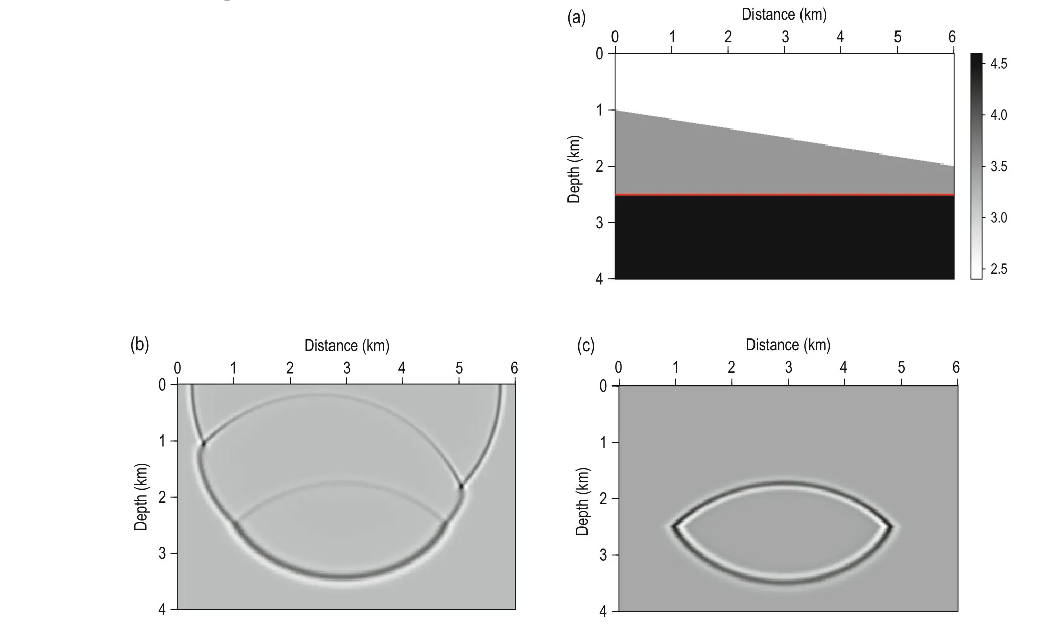
Fig.1 (a) Three-layer velocity model. The velocities of the layers are 2.5 km/s, 3.5 km/s and 4.5 km/s, respectively. The horizontal layer at 2.5 km in depth is stained. (b) The conventional wavefield and (c) the stained wavefield at 1.2 s.

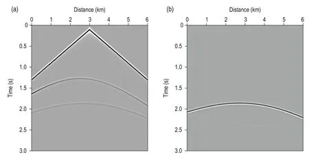
Fig.2 (a) The conventional data and (b) the stained data received on the surface. The source is a Ricker wavelet with a dominant frequency of 15 Hz and time shift of 0.1 s. The source is located at a distance of 3.0 km and the receivers are distributed at every grid on the surface. (c) Reverse-time migration (RTM) imaging result of the conventional data. (d) RTM imaging result of the stained data.

Embedded scattering point method

The constant-density acoustic-wave equation (Symes, 2008) is expressed as:

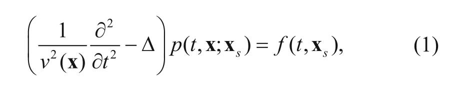
where p(t,x;xs) is the acoustic field, v(x) is the velocity, and f (t, xs) is the source located at xs. To stain the target structure and obtain the stained wavefield and data, we constructed a spatial function for labelling an arbitrary target in the model. Chen and Jia (2014) used the complex domain velocity (CDV) method, which extends all variables in the wave equation to the complex domain. The real part of the complex domain velocity is identical to that of the original velocity model, while, in the imaginary part, a small value is assigned to the target and elsewhere it is zero. The real part of the complex domain wavefield is the conventional wavefield, and the imaginary part is the stained wavefield. Since the CDV method extends the computation to the complex domain, its computational cost is approximately four times that of the conventional real domain computation.

In this study, we used the embedded scattering point (ESP) method to stain the target structure and obtain the stained wavefield and data. In this method, scattering points are embedded into the target structure in the model, i.e., a small velocity perturbation is added to the target structure, and elsewhere it is the same as the original velocity. The distribution of the scattering points is:

where δv(x) is the velocity perturbation and α is the coefficient of perturbation. The stained structure can be an arbitrary structure in the velocity model. The stained wavefield triggered by the scattering points δp(t, x; xs) and the original wavefield together contribute to the total wavefield p(t,x;xs)+δp(t,x;xs). For simplicity, we dropped the variables of time and space. Substituting the velocity containing the scattering points v + δv and the total wavefield p + δp into equation (1), we have the wave equation of the total wavefield expressed as:

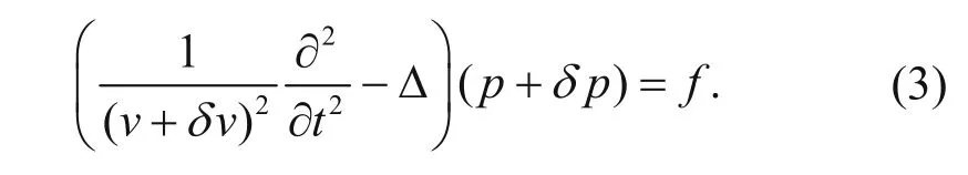
The stained wavefield triggered by the stained structure can be obtained by subtracting equation (1) from equation (3). When the perturbation α is small enough (less than 10% in practical computation), the second-order terms can be dropped, and the stained wavefield is:

Comparing equations (4) and (1), we see that the lefthand side of the equations have the same form, which indicates that the stained and conventional wavefields follow the same equation, i.e., the stained wavefield is synchronized with the conventional wavefield. The right-hand side of equation (4) can be viewed as the source term that triggers the stained wavefield, which is the joint contribution of the target structure and the conventional wavefield. The two equations are the same except for the source term. The conventional wavefield is triggered by the source, while the stained wavefield is triggered by the target structure and the conventional wavefield. Equation (4) indicates that the stained wavefield has the following characteristics: it is not triggered until the wave reaches the target structure, it propagates in synchronization with the conventional wavefield, and it contains only the wavefield related to the target structure. Similarly, the stained data contains only the reflection of the stained target structure. Using the ESP method, we performed the calculation on the models with and without scattering points in the real domain. As such, the computational cost is twice that of conventional modeling, so the cost of the ESP method is half that of the CDV method.

Seismic illumination and resolution analyses

Point spreading function

The seismic image obtained by migration is a distorted description of the actual subsurface structure. The image at location x can be described as a convolution of the PSF and the velocity model (Xie et al., 2005; Cao, 2013; Chen and Xie, 2015):

where I (x) is the image, R (x) is the PSF, m (x) is the velocity model perturbation, and “*” denotes the spatial convolution. Ideally, R (x) can be a δ function, and the image can represent the actual structure. However, due to the illumination issue, R (x) is usually a complex distribution, which smears the image and causes distortion. In the wavenumber domain, equation (5) becomes:

where k is the wavenumber, and I (k), R (k), and m (k) are transforms of I (x), R (x), and m (x), respectively, in the wavenumber domain. Replacing the velocity perturbation m (x) with a point scatter, i.e., a δ function, we have:

In other words, a point scatter image can be seen as the PSF for a given velocity model and acquisition system, and can be used to investigate the effects of the entire system (the acquisition system and overburden velocity) in the imaging process.

We used the ESP method to calculate the stained data from a single scattering point, and used the stained data for the migration to calculate the image of the scattering point, which is also the point spreading function. The process can be described as follows: 1) embed the scattering point in the target, the velocity perturbation is 10%; 2) perform modeling calculation on the model with scattering points and obtain the data D1; 3) perform modeling calculation on the original model and obtain the data D2; 4) subtract D2from D1to obtain the stained data; 5) perform reverse-time migration (RTM) using the stained data on the original velocity model, and obtain the image of the scattering point, which is also the PSF.

Acquisition dip response

The illumination response for a structure with a dipping angle θ is defined as the acquisition dip response (ADR), which can be extracted from the PSF (Chen and Xie, 2015):

where êθis a unit vector along direction θ, c is an arbitrary number, and R (x, k) is the wavenumber domain spectra of the PSF. The integration is along the polar angle θ in the wavenumber domain.

ADR is a function of space and angle, which physically represents how an interface at x with a dipping angle θ can be illuminated by the geometry in the current velocity model (how it can be covered by the seismic energy). It includes the joint effect of the velocity model, geometry, and dipping angle of the target structure. If there is a shadow zone (weak illuminated zone) in the ADR map of a certain angle, the interface with this angle in the zone will not be well illuminated. Thus, a poor imaging result with a weak amplitude and low S/N ratio will be generated. ADR maps illustrate the illumination information of a certain angle of themodel, and provide a tool for estimating the imaging result and improving the image quality by illumination compensation.

Figure 3 shows the ADR calculation process of angle θ using the PSF. Figure 3a shows the PSF of a certain point obtained by the imaging method, assuming that there is an interface with a dipping angle θ (the yellow line) at this point. By transforming the PSF to the wavenumber domain, we obtain the amplitude spectrum of the PSF, as shown in Figure 3b. The spectrum of the interface shown in Figure 3a is an impulse through the origin (the yellow line) in the wavenumber domain. By extracting the energy along θ and integrating the extracted energy, the ADR of the angle can be obtained. Repeating the above operation yields the ADR of the entire model. Because the illumination function is a slow-varying function, we can calculate the PSF in a sparse grid and use interpolation to obtain its value over the entire model.

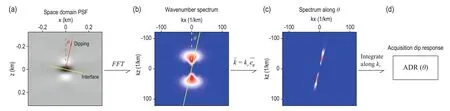
Fig.3 Process for calculating the acquisition dip response (ADR) using the point spreading function. (a) Point spreading function in the space domain. (b) Amplitude spectrum of the PSF in the wavenumber domain. (c) Illumination energy extracted along θ. (d) ADR obtained by integrating the illumination energy along θ.

Image correction

The image is a distorted version of the subsurface structure, and can be expressed as the convolution between the PSF and the structure. The PSF contains all the factors that contribute to the distortion. Once the PSF is eliminated from the image, we can expect to obtain an improved image of the subsurface structure. By deconvolving the PSF from the original image, the distortion can be removed and the image corrected. Deconvolution in the space domain is equivalent to division in the wavenumber domain:

where I (k) and R (k) are the transform of the original image and the PSF in the wavenumber domain, respectively, and I' (k) is the corrected image in the wavenumber domain. Transforming I' (k) to the space domain yields the corrected image. The image correction process is as follows: 1) choose a proper window function for sampling the localized original image and the corresponding PSF; 2) transform the localized space domain image and PSF to the wavenumber domain, divide the spectrum of the PSF from from the spectrum of the image, and transform the corrected spectrum back to the space domain; 3) repeat the operation for the entire model to obtain the corrected image.

Numerical experiments

The source for all the experiments in this section is a Ricker wavelet with a dominant frequency of 15 Hz and time shift of 0.1 s.

Figure 4 shows a comparison of the stained data from a single scattering point obtained by the CDV and EPS methods. We used the model shown in Figure 1a for the calculation. The source is located 3.0 km away, and the receivers are distributed at every grid on the surface. The grid size is 0.01 km, and the scattering point is at a distance of 3.0 km and a depth of 2.0 km. The stained data obtained by the CDV and EPS methods are shown in Figures 4a and 4b, respectively. The results obtained by the two methods appear to be the same, except for their orders of magnitude. Figures 4c and 4d show the traces of synthetic seismograms recorded at a distance of 3.0 km on the surface by the two methods, respectively, with the amplitudes normalized. Figure 4e shows the difference between the two normalized traces, which is effectively zero compared with the original traces.Apart from their orders of magnitude, the stained data obtained by the two methods have the same travel time and waveform. Thus, the two methods can be seen to be equivalent in the calculation of the stained data.

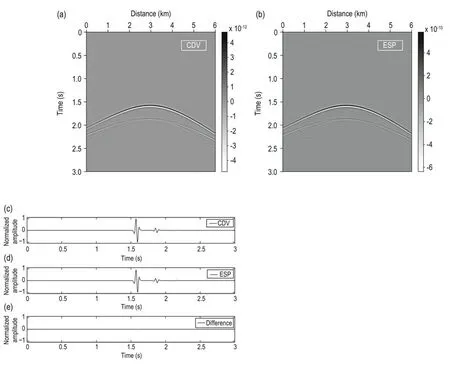
Fig.4 Stained data from a single scattering point obtained by (a) CDV method and (b) ESP method. The scattering point is at a distance of 3.0 km and 2.0 km in depth in the model shown in Fig. 1a. The source is located at a distance of 3.0 km, and the receivers are distributed at every grid on the surface. (c) Normalized trace of (a) recorded at a distance of 3.0 km on the surface. (d) Normalized trace of (b) recorded at a distance of 3.0 km on the surface. (e) The difference between (c) and (d).

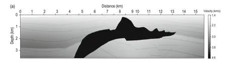
Figure 5 shows the PSFs obtained by the staining algorithm in a complex media. Figure 5a shows the SEG salt model results, where the subsalt area is the zone of interest and the challenge for imaging. The receivers are to the left of the source with the largest offset of 4.27 km, and the intervals of the receivers and shots are 0.024 km and 0.049 km, respectively. We used the ESP method to calculate the stained data, and the spike array is 0.1 km × 0.1 km with a velocity perturbation of 10%. The top panel of Figure 5b shows the space-domain PSFs obtained by imaging the sc attering points using the stained data. The wavenumber-domain amplitude spectra of the PSFs at selected locations are shown in the bottom panel. The distributions of the spectra vary at different locations. In the non-subsalt areas, the spectra have a broad distribution, which indicate that reflectors with various dipping angles can be well illuminated. Conversely, in the subsalt area, the spectra are distributed within a narrow angle, which indicates that only the reflectors with a dipping angle restricted to this narrow range can be illuminated. In addition, the illuminated ranges vary with locations in the subsalt area.

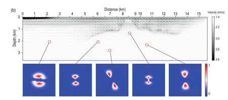
Fig.5 SEG salt model. Top: space-domain PSFs. The interval of the spike array is 0.1 km. Bottom: amplitude spectra of the PSFs in the wavenumber domain in selected locations.

Figure 6 shows the ADRs for various angles of the SEG salt model, which clearly reveal that, in the subsalt shadow zone, the illuminations of different dipping angles behave differently. Reflectors with a dipping angle of -15° can be well illuminated (as shown in Figure 6a), while those with a dipping angle of 45° cannot be illuminated (shown in Figure 6d). This indicates that the geometry in the current velocity model can be used to detect the -15°-dipping-angle reflector effectively, but not the 45°-dipping-angle reflector. Since the dipping angle of the reflector in the subsalt area is 45°, this explains why it cannot be imaged well.

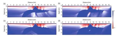
Fig.6 ADRs for selected dip angles of (a) -45° (b) -15° (c) 15° and (d) 45° in the SEG salt model.

Figure 7 shows the image correction by PSF deconvolution, with Figure 7a showing the original prestack depth image. The red square indicates the size of the spatial sampling window for correction. From the left to the right in Figure 7b are the localized original image, point spreading function, image spectrum, PSF spectrum, and corrected image, respectively. By repeatedly using the PSF to deconvolve the entire image, we obtain the corrected image shown in Figure 7c. Compared with the original image, the correction significantly enhances the structure and reduces the artifacts. The biased image from the joint effect of uneven illumination and complex subsurface structure has been corrected.

Figure 8 shows the spectra analyses results for the original and corrected images. The middle panel shows the reflectors overlapped by the vertical profiles extracted from five locations. The red and blue lines represent the profiles of the original and corrected images, respectively. The profiles from the surface to 0.24 km in depth are muted to better illustrate the details. The results reveal that the reflectors are well extracted inthe corrected image, especially in shallow sediments, e.g., at 11 km in distance. The top panel shows the amplitude spectra of the vertical wavenumber, which reveals that the low-wavenumber components are well suppressed, and the high-wavenumber components are enhanced. We selected two zones in the figure (indicated by the green dashed squares) to further illustrate the correction. The left zone contains simple layered structures, while the right contains a salt body with a complex boundary. The original and corrected images and the corresponding amplitude spectra in the wavenumber domain are shown in the bottom panel. The results reveal that the salt boundary and the layers above the salt are sharper and clearer in the corrected image. All the reflectors are “stripped” of low-wavenumber artifacts, which are illustrated in the wavenumber-domain spectra analysis results. The average spectra distributions of the corrected images in both zones shift to higher wavenumbers. Consequently, the 1D and 2D spectra analysis results show that the resolution and quality of the corrected image are significantly improved.

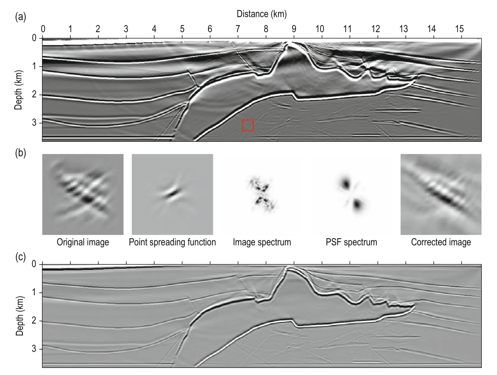
Fig.7 Image correction by PSF deconvolution.

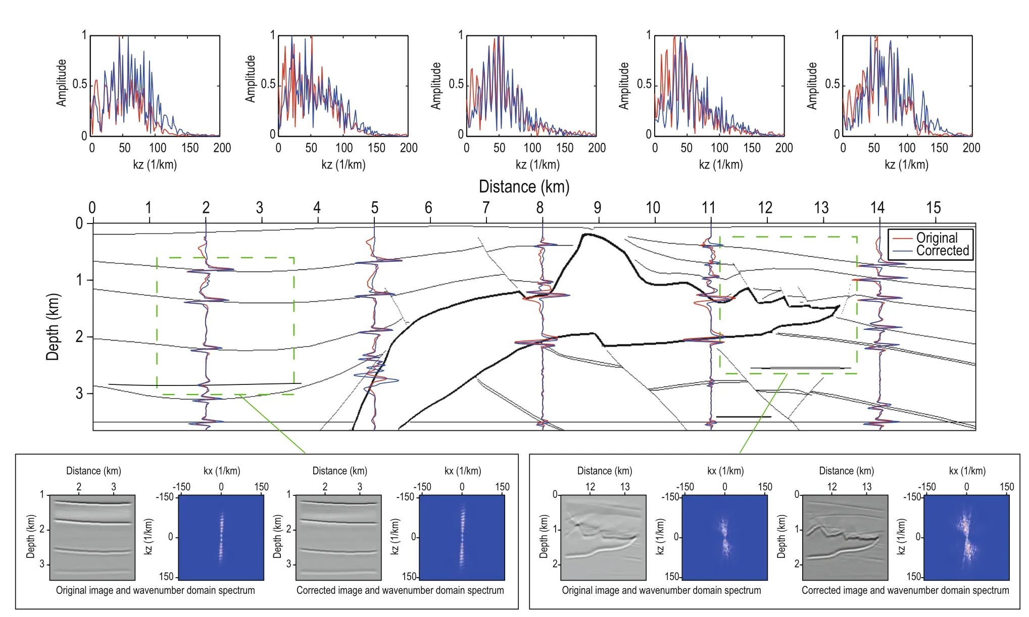
Fig.8 The original and corrected image and the corresponding amplitude spectra in wavenumber domain.

Conclusions

Seismic illumination and resolution analyses provide a quantitative description of how an image is distorted. The point spreading function indicates the resolution of the depth image and carries full information about the factors affecting the quality of the image. We used the staining algorithm to establish the correspondence between a certain structure and its relevant wavefield and reflected data. We calculated the PSF by imaging a scattering point using the scattered data obtained by the staining algorithm, and extracted broadband illumination information from the amplitude spectra in the wavenumber domain of the PSF. The following conclusions can be drawn:

1) The ESP and CDV methods yield the same normalized stained data, and the computation costs in time of the ESP method is half that of the CDV method.

2) The calculation of the PSF is based on a full-wave equation and contains broadband information. The related information extracted from the PSF contains the broadband effect, and thus better describes the characteristics of illumination and resolution.

3) Angle domain illumination information can be obtained by extracting the amplitude spectra of the PSF in the wavenumber domain.

4) By deconvolving the PSF from the original image, the biased image from the joint effect of uneven illumination and complex subsurface structure can be corrected.

Acknowledgements

The authors thank Hu Jinyin and Li Qihua for their fruitful discussions and suggestions for the manuscript. We also thank Profs. Hu Tianyue and Liu Jiancheng for their valuable comments and constructive suggestions.

Bear, G., Liu, C. P., Lu, R., et al., 2000, The construction of subsurface illumination and amplitude maps via ray tracing: The Leading Edge, 19(7), 726-728.

Cao, J., 2013, Resolution/illumination analysis and imaging compensation in 3D dip-azimuth domain: 83rd Annual International Meeting, SEG, Expanded Abstracts, 3931–3936.

Cao, J., and Wu, R. S., 2009, Full-wave directional illumination analysis in the frequency domain: Geophysics, 74(4), S85–S93.

Chen, B., and Jia, X., 2014, Staining algorithm for seismic modeling and migration: Geophysics, 79(4), S121–S129.

Chen, B., Ning, H., and Xie, X. B., 2016, Investigating the effect of shallow scatterings from small-scale nearsurface heterogeneities to seismic imaging: A resolution analysis based method: Chinese J. Geophys. (in Chinese), 59(5), 1762-1775.

Chen, B., and Xie, X. B., 2015, An efficient method for broadband seismic illumination and resolution analyses:85th Annual International Meeting, SEG, Expanded Abstracts, 4227-4231.

Dale, L., and Slack, J. M. W., 1987, Fate map for the 32-cell stage of Xenopuslaevis: Development, 99, 527–551.

Gelius, L. J., Lecomte, I., and Tabti, H., 2002, Analysis of the resolution function in seismic prestack depth imaging: Geophysical Prospecting, 50, 505–515.

Gilbert, S. F., 2000, Developmental Biology: Sinauer Associates, Sunderland (MA), 265-268.

Ginhoux, F., M., Greter, M., Leboeuf, S. et al., 2010, Fate mapping analysis reveals that adult microglia derive from primitive macrophages: Science, 330, 841–845.

Jackson, M. P. A., Vendeville, B. C., and Schultz-Ela, D. D., 1994, Salt-related structures in the Gulf of Mexico: A field guide for geophysicists: The Leading Edge, 13, 837–842.

Lecomte, I., 2008, Resolution and illumination analyses in PSDM: A ray-based approach: The Leading Edge, 27, 650–663.

Leveille, J., Jones, I., Zhou, Z., Wang, B., and Liu, F., 2011, Subsalt imaging for exploration, production, and development: A review: Geophysics, 76(5), WB3–WB20.

Liu, Y., Chang, X., Jin, D., He, R., Sun, H., and Zheng, Y., 2011, Reverse time migration of multiples for subsalt imaging: Geophysics, 76(5), WB209–WB216.

Luo, M., Cao, J., Xie, X. B. et al., 2004, Comparison of illumination analyses using one-way and full-wave propagator: 74th Annual International Meeting, SEG, Expanded abstract, 67-70.

Mao, J., and Wu, R. S., 2011, Fast image decomposition in dip angle domain and its application for illumination compensation: 81st Annual International Meeting, SEG, Expanded Abstracts, 3201-3204.

Muerdter, D., and Ratcliff, D., 2001, Understanding subsalt illumination through ray-trace modeling, Part 1: Simple 2-D salt models: The leading Edge, 20(6), 578-594.

Symes, W. W., 2008, Migration velocity analysis and waveform inversion: Geophysical prospecting, 56(6), 765–790.

Valenciano, A., Lu, S., Chemingui, N. et al., 2015, High resolution imaging by wave equation reflectivity inversion: 77th Annual International Conference and Exhibition, EAGE, Extended Abstracts, We N103.

Wu, R. S., and Chen, L., 2006, Directional illumination analysis using beamlet decomposition and propagation: Geophysics, 71(4), S147–S159.

Wu, R. S., Chen L., and Xie, X. B., 2003, Directional illumination and acquisition dip-response. 65th Conference and Technical Exhibition, EAGE, Expanded abstract, P147.

Wu, R. S., Xie, X. B., Fehler, M., and Huang, L. J., 2006, Resolution analysis of seismic imaging: 68th Annual International Conference and Exhibition, EAGE, Extended Abstracts, G048.

Xie, X. B., Jin, S. W., and Wu, R. S., 2006, Wave-equation based seismic illumination analysis: Geophysics, 71(5), S169–S177.

Xie, X. B., Wu, R. S., Fehler, M., and Huang, L., 2005, Seismic resolution and illumination: A wave-equation based analysis: 75th Annual International Meeting, SEG, Expanded Abstracts, 1862–1865.

Xie, X. B., and Yang, H., 2008, A full-wave equation based seismic illumination analysis methods: 70th Annual International Conference and Exhibition, EAGE, Extended Abstracts, P284.

Yan, R., Guan, H., Xie, X. B., and Wu, R. S., 2014, Acquisition aperture correction in the angle domain toward true-reflection reverse time migration: Geophysics, 79(6), S241-S250.

Yang, H., Xie, X. B., Jin, S., and Luo, M., 2008, Target oriented full-wave equation based illumination analysis: 78th Annual International Meeting, SEG, Expanded Abstracts, 2216-2220.

Chen Bo, PhD candidate in geophysics of University of Science and Technology of China. Graduated in 2010 and obtained B.S. from USTC. Now works on seismic wave propagation and seismic imaging for complex media at University of Science and Technology of China, School of Earth and Space Sciences. Email: chenbo6@mail.ustc.edu.cn

Manuscript received by the Editor April 7 2016; revised manuscript received May 30, 2016.

*This study was funded by the National Natural Science Foundation of China (No. 41374006 and 41274117).

1. University of Science and Technology of China, School of Earth and Space Sciences, Laboratory of Seismology and Physics of Earth’s Interior, Hefei Anhui 230026, China.

2. Institute of Geophysics and Planetary Physics, University of California at Santa Cruz, CA 95064, U.S.A.

3. School of Earth Science and Geological Engineering, Sun Yat-sen University, Guangzhou 510275, China.

♦Corresponding author: Jia Xiao-Feng (Email: xjia@ustc.edu.cn)

© 2016 The Editorial Department of APPLIED GEOPHYSICS. All rights reserved.