Spherical cap harmonic analysis of regional magnetic anomalies based on CHAMP satellite data*

Feng Yan, Jiang Yong, Jiang Yi, Liu Bao-Jia, Jiang Jin, Liu Zhong-Wei, Ye Mei-Chen, Wang Hong-Shen, and Li Xiu-Ming

Spherical cap harmonic analysis of regional magnetic anomalies based on CHAMP satellite data*

Feng Yan♦1,2, Jiang Yong1, Jiang Yi1, Liu Bao-Jia1, Jiang Jin1, Liu Zhong-Wei1, Ye Mei-Chen1, Wang Hong-Shen1, and Li Xiu-Ming1

We used CHAMP satellite vector data and the latest IGRF12 model to investigate the regional magnetic anomalies over mainland China. We assumed satellite points on the same surface (307.69 km) and constructed a spherical cap harmonic model of the satellite magnetic anomalies for elements X, Y, Z, and F over Chinese mainland for 2010.0 (SCH2010) based on selected 498 points. We removed the external field by using the CM4 model. The pole of the spherical cap is 36N° and 104°E, and its half-angle is 30°. After checking and comparing the root mean square (RMS) error of ΔX, ΔY, and ΔZ and X, Y, and Z, we established the truncation level at Kmax= 9. The results suggest that the created China Geomagnetic Referenced Field at the satellite level (CGRF2010) is consistent with the CM4 model. We compared the SCH2010 with other models and found that the intensities and distributions are consistent. In view of the variation of F at different altitudes, the SCH2010 model results obey the basics of the geomagnetic field. Moreover, the change rate of X, Y, and Z for SCH2010 and CM4 are consistent. The proposed model can successfully reproduce the geomagnetic data, as other data-fitting models, but the inherent sources of error have to be considered as well.

Geomagnetic model, CHAMP satellite, spherical cap harmonic model, CM4, IGRF12

Introduction

Geomagnetic satellites (geomagnetic field measurement satellites) offer high precision and continuous coverage, and since the launch of Sputnik-3, first geomagnetic satellite, large numbers of satellite data have been amassed. Global or regional geomagnetic models are based on satellite data because of the high quality and dense distribution of the data that allow to investigate the secular variations of the geomagnetic field.

The CHAMP satellite was launched in July 2000 from the Plesetsk satellite base in Russia to near-polar, circular orbit at altitude of 454 km to collect geomagnetic and gravity data. The three vectors (north, east, and vertical) were measured by a Fluxgate magnetometer.The scalar (total intensity F) was measured by using an Overhauser magnetometer, and the satellite attitude was calculated by a pair of star sensors (Hemant and Maus, 2003; Mandea and Puruker, 2005). The absolute error is less than 0.5 nT. Maus et al. (2002) first derived the global scalar anomalies distribution. Subsequently, after combining with ground-based data, more global highprecision geomagnetic models began to emerge, such as the geomagnetic field comprehensive model series (Sabaka et al., 2004, 2015), the CHAOS model series (Olsen et al., 2010, 2014), the MF model series (Maus et al., 2008), and the NGDC-720 model (Maus, 2010). These models describe the distribution of the main and lithospheric fields as well as the temporal and spatial variation of external fields.

Regional-scale studies combine data and regional models, such as Taylor series, spherical cap harmonics (Haines, 1985), surface splines (An and Xu, 1981), rectangular harmonics (Alldredge et al., 1981), Legendre polynomials, and many others.

The spherical cap harmonic (SCH) model is a model of an area in the spherical cap coordinate system. Compared with other regional models, the SCH model has two advantages. It satisfies the geomagnetic potential theory and describes the three-dimensional structure of the geomagnetic field. Haines (1985) analyzed the geomagnetic variations in Canada during 1960-1983 by using the SCH model. An et al. (1998) and An (2000) analyzed the anomalies over the Qinghai–Tibet Plateau and Europe by using the SCH model and satellite data. Chen et al. (2011) studied the geomagnetic field and its secular variations over China by using the SCH model. In addition, Thébault et al. (2004) modified the SCH model by replacing the monotonic exponential function to improve the fitting of the geomagnetic radial elements, and the modified SCH (RSCH) model by combining repeat stations, observatories, and aerial and CHAMP satellite data. Thébault (2006) also analyzed the lithospheric field over France. Ou et al. (2013) studied the lithospheric field over China by using surface and satellite data and the RSCH model. The abovementioned studies demonstrated the correlations between magnetic anomalies and geological structures.

Despite the work on the regional geomagnetic field over China, the full advantage of the CHAMP data at satellite altitude has not taken place. Considering that the SCH model can express the regional anomalies, we chose the SCH model and select CHAMP data to model the magnetic anomalies in China and compared the results with other models. To some extent, this study covers the temporal and spatial distribution of the lithospheric field over China and East Asia. In section two, we discuss the treatment of the satellite data and SCH model. In section three, we describe the results, and the discussion and conclusions are given in the last two sections.

Data and methods

CHAMP satellite data

All satellite data are taken from the Helmholtz Center at the Potsdam German Research Center for Geosciences (GFZ) (http://www.gfz-potsdam. de/startseite/) and compriselevel-1 scalar data from the Overhauser magnetometer (OVM) and Fluxgate magnetometer (FGM). Owing to changes in location and intensity during data collection, time calibration, data transformation, temperature treatment, and other transformations are needed to obtain level-2 data, which cannot be used directly until the FGM frame data are transferred to the NEC (north, east, and center) frame data (Flechtner et al., 2010). These operations are done according to the following sequence

The steps described by equation (1) are listed in Table 1.

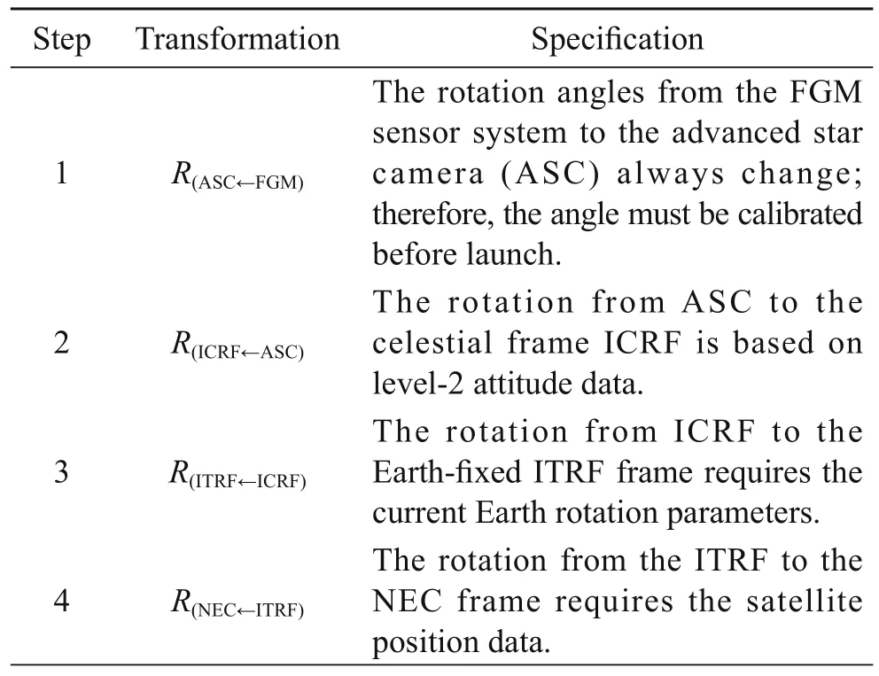
Table 1 FGM frame to NEC frame data

Subsequently, we performed the time transformation according to the following criteria.

1) Select data during 18: 00–23: 00 LT and 00: 00–5: 00 LT night-side data;

2) Select data when Kp ≤ 2;

3) Select the data when |Dst| ≤ 20 nT.

Considering that the magnetic anomalies are nearly time-independent, we analyzed the geomagnetic field over China in 2010.0 (1/1/2010) for the region within 18°N-54°N and 73°E-136°E. To obtain an ideal and dense satellite data distribution, we consider the midday data for 60 days. Each point is weighted the same, which allows to calculate the mean value at each 1°grid square. For the rest of the points, piecewise interpolation is adopted. To decrease the difference between adjacent tracks, ascending data were chosen (Maus et al., 2006). Next, we take 2010.0 as the study points at 1° intervals and perform gridding and piecewise interpolation. Finally, 2368 satellite grid points were obtained for the study region. For convenience, we then selected 400 grid points within the boundaries. To avoid the boundary effects in the numerical simulations, we selected 98 satellite points outside the boundaries by the UA method (Feng et al., 2015). The final model was based on 498 points. Because 2010 was the last observation year for CHAMP, the orbit altitude decreased and all points were in the range 302.59-312.84 km.

The biggest altitude difference among satellite points is 3.3% (around 10 km). We also assumed that all points are at the same surface (307.69 km), which is the average altitude. Thus, the model was based on 498 data at the same level (307.69 km).

Spherical cap harmonic model

The magnetic anomaly model for 2010.0 was based on the SCH model, which is typically adopted to simulate regional magnetic anomalies (ΔX, ΔY, ΔZ) at satellite level. The model was constructed by subtracting the main field values from the latest generation of the International Geomagnetic Reference Field (IGRF) data—IGRF12 for all 498 measured values. All magnetic anomalies were expressed (Haines, 1985) as follows:

We used the fourth geomagnetic comprehensive model (CM4) to remove the time-dependent weak external magnetic fields, such as the ionospheric and magnetospheric field and their induced fields as well as the toroidal field at satellite level with intensities less than 1% of the total intensity, to obtain the magnetically anomalous data.

Results

Truncation level

The SCH model is a data-fitting model similar to Taylor series and rectangular harmonic models; thus, the truncation level has to be determined. If the level is low, the fitting is not good, which will result in low precision and, if the level is high, the calculations are time-consuming. Moreover, the Runge phenomenon may occur with increasing level and artifacts may be generated.

The criteria to choose the truncation level are two. The root mean square error (RMS) must be less than that of IGRF to obtain a good regional model, and the RMS must be stable while the level increases (An, 2001). After obtaining the model anomalies, we calculated the RMS based on the actual anomalies by subtracting the IGRF from the data. In Figure 1, we show the variation of RMS for ΔX, ΔY, and ΔZ as a function of the truncation level (Kmax).

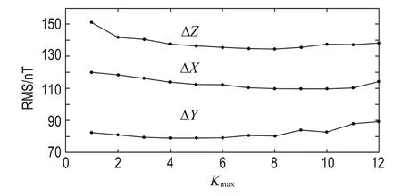
Fig.1 RMS (nT) for ΔX, ΔY, and ΔZ vs Kmax.

In Figure 1, we see that the RMS for ΔX, ΔY, and ΔZ gradually decreases with increasing Kmaxup to six, is stable up to ten, and then slightly increases, especially for ΔY. To determine the truncation level, we calculated the RMS between the total field (sum of model anomalies and IGRF) and the measurements, and showthe variation as a function of Kmaxin Figure 2.

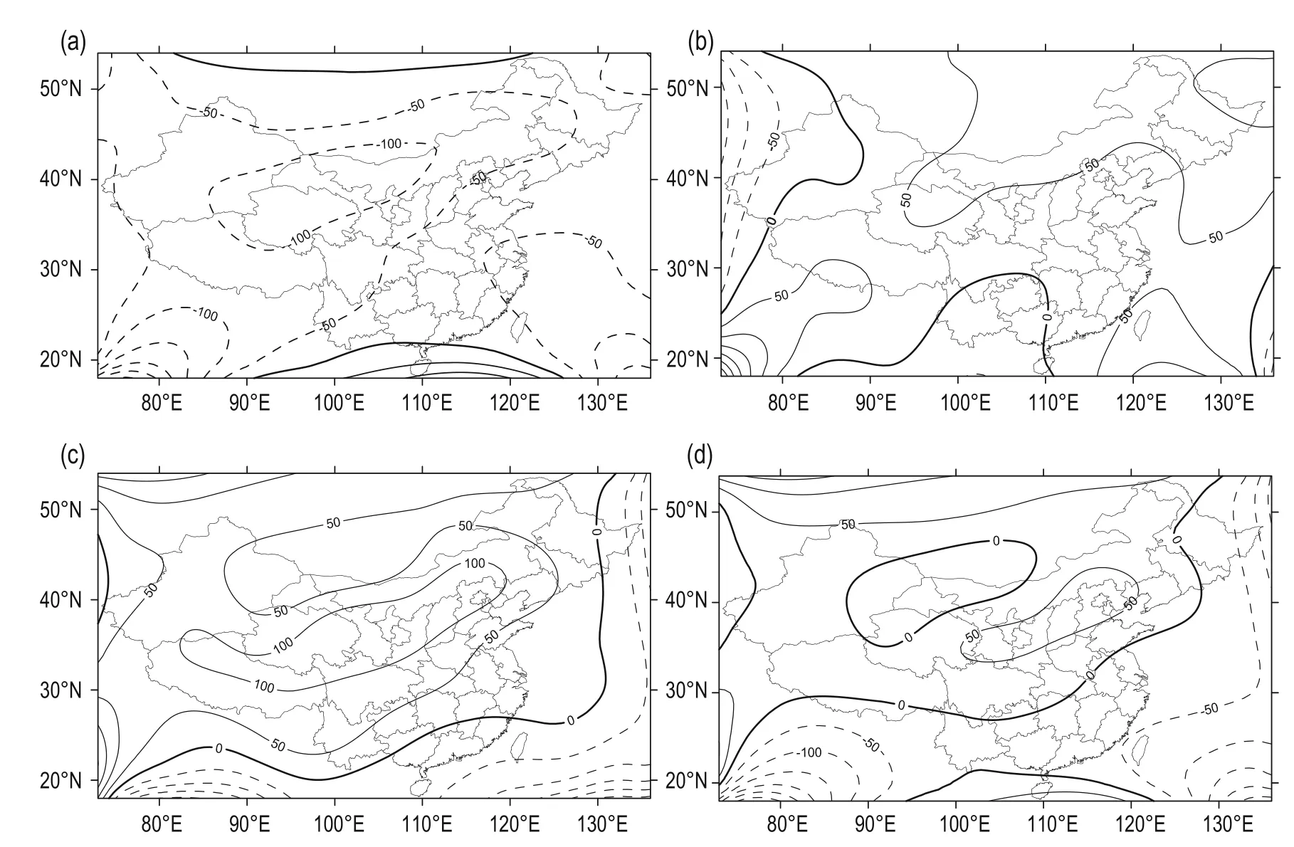
Fig.3 Satellite magnetic anomalies over the Chinese mainland based on the SCH2010 model with Kmax= 9. (a)-(d): elements X, Y, Z, and F. Unit: nT.

In Figure 2, the RMS for X, Y, and Z sharply decrease for Kmax= 1-8 by 96.37%, 92.43%, and 95.88%, respectively, and are stable from Kmax= 8 onward. Considering the first criterion, we established the RMS for X, Y, and Z based on IGRF12 as 150.70 nT, 131.40 nT, and 212.86 nT, respectively. Using the other two criteria and the calculation cost, we take Kmax= 9 as the truncation level.

Fig.2 RMS for X, Y, and Z vs Kmax.

The derivation of SCH2010

After determining Kmax, we created magnetic anomalies models for China at the satellite level of 2010.0. We next show and list the gridded anomalous figures of elements X, Y, Z, and F (Figure 3) at spatial resolution of 1° (about 111.12 km).

Compared to the main field, the anomalous field is small and accounts for about 4% of geomagnetic field. The distribution of the anomalous field is spatially complex but temporally stable. Magnetic anomalies attenuate sharply with increasing radial distance; thus, the anomalies at satellite level are generally smaller than near the surface. In Figure 3, X is negative inside the boundary and there is an extreme point around -150 nT at the intersection of Yunnan, Gansu, and Inner Mongolia. Y is positive in most parts, and the intensity increases from 0 nT to around 70 nT with increasing latitude. Z and F are, to some extent, similar. Z is positive, except in Hainan, Guangdong, South Fujian, and South-East Yunnan, with an extreme point around 130 nT in central China and increasing intensity from 0 nT to around 130 nT and then decreasing to around 20 nT with decreasing latitude. For F, the areas above the zero-contour line near 30° N are positive and negative below, and there is an extreme point around 70 nT in the Beijing region and another one around -30 nT at the intersection of Xinjiang, Gansu, and Inner Mongolia.

Based on SCH2010 and IGRF12, we obtain the 2010 Chinese Geomagnetic Reference Field at satellite level (Kmax= 9)—CGRF2010 is obtained with the equation CGRF2010 = IGRF2010+SCH2010. The distributions of X, Y, Z, and F based on CGRF2010 are shown in Figure 4.

Fig.4 Geomagnetic field distribution over the Chinese mainland at satellite level based on the SCH2010 model. (a)–(d): X, Y, Z, and F. Unit: nT

We compare Figure 4 with other models, such as CM4 and CHAOS3, and find that the distribution and intensity are consistent and reflect the actual geomagnetic field over China, which suggests that the proposed model is reliable.

Comparison with different models

To verify the SCH2010 model, we calculated its gridded values. The anomalies are temporally stable and thus their distribution does not change with time. We compare our results with those of An (2003) (SCH1936 and Kmax= 8). Figure 5 shows the distribution of ground magnetic anomalies for X, Y, Z, and F based on the two models.

Based on the compared distributions of the magnetic anomalies, we found that the distributions and intensities of the four elements in both models are very similar. For X, the distribution is negative. There are two anomalous regions in Southwest Inner Mongolia and Northeast Inner Mongolia, with extreme points around -300 nT and -200 nT, respectively. These two anomalies connect and form a saddle-shaped region. The distribution for Y is positive and negative. There are saddle-shaped positive regions in Qinghai, Gansu, and Inner Mongolia. The distribution of Z is positive, with saddle-shape regions in Southwest Qinghai and Northeast Inner Mongolia and two extreme points around 250 nT. Like Z, F has a similar saddle-like distribution but with weakerextreme points and an anomalous region north of the saddle region with an extreme point around -200 nT. SCH2010 and SCH1936 yield similar results, which supports the proposed model.

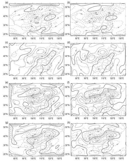
Fig.5 Distribution of magnetic anomalies at the surface for SCH1936 (left column) and SCH2010 (right column). (a) and (b): X; (c) and (d): Y; (e) and (f): Z; (g) and (h): F. Unit: nT.

To inspect the spatial variation of SCH2010, we examine the distributions at 100 km, 200 km, and 300 km and use F as an example (Figure 6).

The anomaly of F decreases with increasing altitude. According to Figure 6, the shape of the anomaly at the ground is relatively complex; north of the zero-contourline is negative and south of it is positive. There are two positive regions in western Tibet and southern Yunnan. At 100 km, the anomaly is simpler, with two anomalous regions near the zero-contour line but their intensities have decreased to about 50 nT; however, the positive region near Yunnan has disappeared. At 200 km, the two anomalous regions and their intensities further decrease, and the positive region near Tibet has disappeared. At 300 km, two closed contour lines replace the two anomalous regions, and it is hard to see any anomalies. From the surface up to 300 km, the zero-contour line is almost fixed; however, the absolute intensity of the other anomalies decreased to about 150 nT and the shapes have significantly simplified.

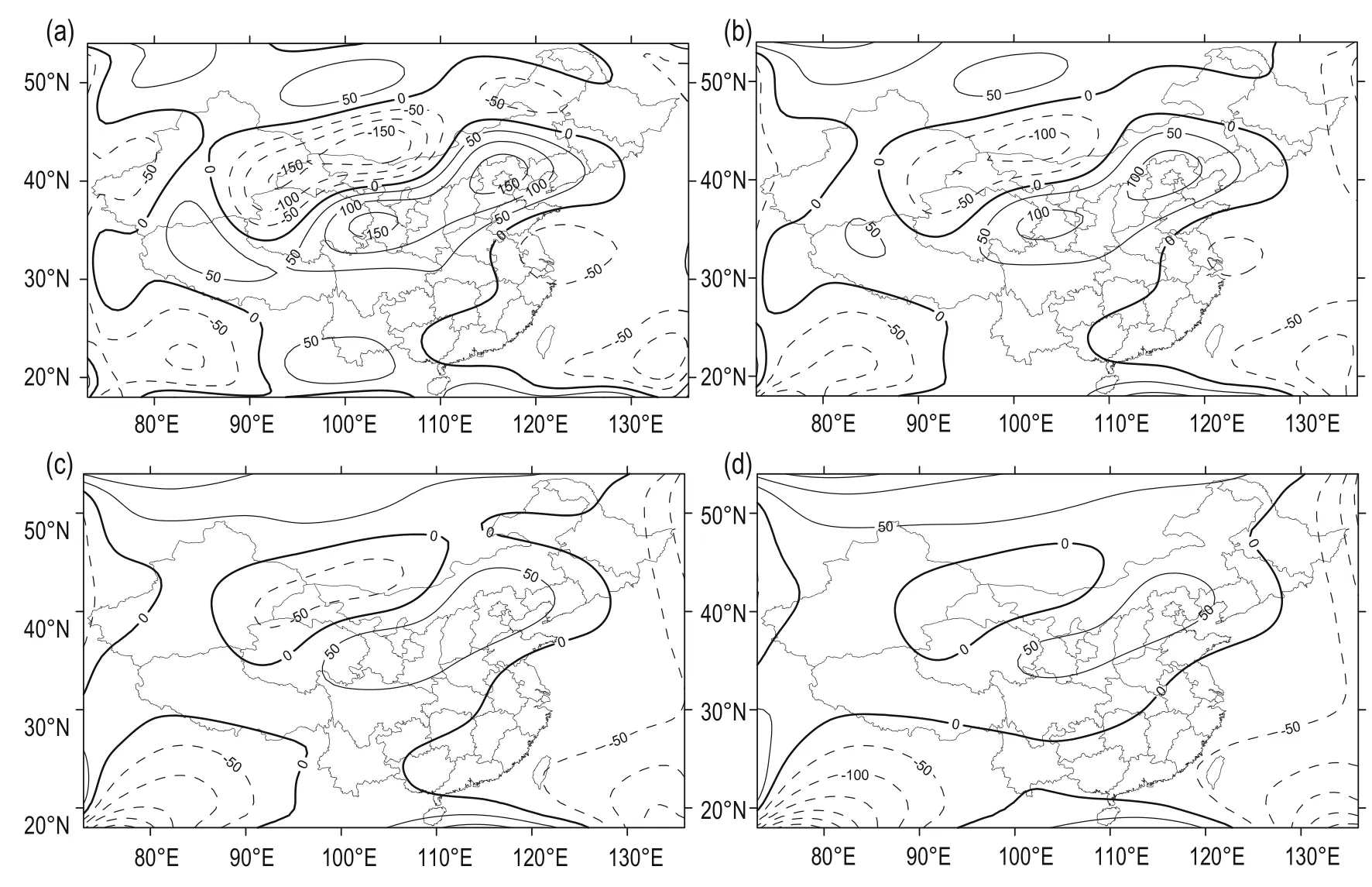
Fig.6 Magnetic anomalies distribution of F based on SCH2010. The contour interval is 50 nT. (a): 0 km (surface); (b): 100 km; (c): 200 km; and (d): 300 km. Unit: nT.

Discussion

To inspect the spatial variations of SCH2010, two points (120°E, 29°N) and (104°E, 36°N) were randomly selected. The latter is at the center of the study region and the former lies in central Zhejiang and close to a negative extreme point. In Figure 7, the distributions of X, Y, and Z at 100 km, 200 km, and 300 km are shown for SCH2010 and CM4, respectively.

According to Figure 7, the changes of the three elements at the two points for the two models are basically the same, which is consistent with the results in Feng et al. (2013). The intensity of X decreases with increasing altitude by about 0.73% and 0.98%, and 9.50% and 10.42% on average from the surface to 300 km for SCH2010 and CM4, respectively. Y increases with increasing altitude but the two models show decreased intensities by 2.13% and 2.86% on average at 120°E, 29°N and increased intensities by 34.44% and 36.81% on average at 104°E, 36°N. The same is seen for Z; the intensities increased by 12.78% and 12.68% on average at 120°E, 29°N but decreased by 18.01% and 19.19% on average at 104°E, 36°N. The change rates of the three elements at the different altitudes agree and the generated differences are attributed to the local magnetic anomalous intensities and attenuation rates. For Y and Z, the change trends are the same. Obviously, there is good agreement between SCH2010 and the global model.

The errors of the SCH2010 are attributed to the following sources. First the model itself, the SCH model is based on the residual field after removing the main or the dipole field. The advantage of this is that the applied least squares method is not ill conditioned and an effective numerical solution is obtained. However, errors still exist when the distribution of the measured points isuneven. Many studies have shown that by increasing the spherical cap half-angle we can improve the accuracy. It is well known that the SCH model can better model the long-wavelength parts of the lithospheric field owing to it slow spatial resolution. Hence, the middle-wavelength parts are not modeled well and this causes problems (Xu et al., 2011). These problems have been dealt with the revised SCH model (Thébault et al., 2004) and for regions with little or no data the SCH model gives better results.

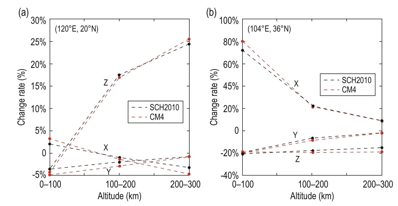
Fig.7 The change rate of magnetic elements for SCH2010 and CM4.

During modeling, a truncation error is inevitably present regardless of the method used; therefore, a better approach is to suppress it by referencing the RMS. By comparing the proposed model with global models, such as CHAOS3 and EMM2010, we found that the distributions of X and Z are simple but differ with the corresponding distributions of the global models. This is likely due to the grid processing of the satellite data; moreover, the radial function (Z direction) of the SCH model does not model the change in the geomagnetic field.

The analysis of the satellite anomalies involves not only the distribution of points but also the altitude. In addition, the limitations of the electromagnetic potential field should be considered. This means that the internal magnetic field is presumably a source-free field (divergence and curl are zero), which makes the SCH model well suited for this type of analysis. In theory, the SCH model can handle the middle-wavelength field data (An and Tan, 1998) but not the short-wavelength data. Nevertheless, the SCH model is widely used in regionalscale studies. Considering its properties and errors, more surface data should be included in future models. Although the surface data are more uneven than the satellite data, they are of higher precision and density. The coefficients of the SCH model that are based on two kinds of data better express the spatial variation of the magnetic field. For regions with large anomalies, more data can be included (INTERMAGNET chains and satellite data) to improve the precision.

Conclusions

We constructed a magnetic anomaly model, SCH2010, for China based on CHAMP gridded data, and the IGRF12 and CM4 models.

A suitable truncation level needs to be obtained when simulating the regional magnetic field. The SCH model is generally based on the anomalous values; thus, it is better to use the RMS and the distribution of the anomalies.

The distribution of the anomalies at the satellite level is relatively simple. For X, it is negative over China, whereas for Y, Z, and F is positive. There is good consistency between CGRF and the proposed model based on IGRF12 and CM4. The shapes for SCH2010 at the surface and that of SCH1936 are highly consistent. The magnetic field results for F at different altitudes suggest that the variation of the anomalous field with altitude follows the laws of the geomagnetic field.

Compared to a Taylor series model, the SCH2010 with nine degrees of freedom has more curved contour lines and more anomalous regions. In addition, by removing the external fields, the SCH2010 better models the satellite anomalies over China.

To inspect the spatial variation of SCH2010, twopoints (120°E, 29°N) and (104°E, 36°N) were randomly selected. The latter is the center point of the study region and the former lies in the central Zhejiang and close to a negative extreme point. The distributions of X, Y, and Z at 100 km, 200 km, and 300 km is shown for SCH2010 and CM4.

Acknowledgements

We acknowledge the support of the staff of the State Key Laboratory of Space Weather, Chinese Academy of Sciences. We also wish to thank reviewers Zhang Suqin, Huang Ya, and Mao Fei for their constructive comments.

Alldredge, L. R., 1981, Regional harmonic analyses applied to the geomagnetic field: J. Geophys. Res., 86(B4), 3021 -3026.

An, Z. C., 2000, Studies on geomagnetic field models of Qinghai-Xizang plateau: Chinese J. Geophys., 43(3), 339 -345.

An, Z. C., 2001, Analyses and discussions of the geomagnetic field polynomial models: Chinese J, Geophys., 27(6), 511-522.

An, Z. C., 2003, Spherical cap harmonic model of the Chinese geomagnetic reference field for 1936: Chinese J. Geophys., 46(5), 624-627.

An, Z. C., Rotanova, N. M., Odintsov, S. D., et al., 1998, Spherical cap harmonic models of MAGSAT magnetic anomalies over Europe and its adjacent region: Chinese J. Geophys., 41(4), 468-474.

An, Z. C., and Tan, D. H., 1998, Spherical cap harmonic analysis of MAGSAT magnetic anomalies over Asia: Chinese J. Geophys., 41(2), 168-173.

An, Z. C., and Xu, Y. F., 1981, Methods of computation of geomagnetic field at greater altitude in a local region: Chin. J. Space Sci., 1(1), 68-73.

Chen, B., Gu, Z. W., Gao, J. T., et al., 2011, Analyses of geomagnetic field and its secular variation over China for 2005.0 epoch using spherical cap harmonic method: Chinese J. Geophys., 54(3), 771-779.

Feng, Y., Sun, H., Jiang, Y., 2015, Data fitting and modeling of regional geomagnetic field: Applied Geophysics, 12(3), 303-316.

Flechtner, F. M., Gruber, T., Guntner, A., et al., 2010, System earth via geodetic-geophysical space techniques: Springer-Verlag, Berlin.

Haines, G. V., 1985, Spherical cap harmonic analysis: J. Geophys. Res., 90(B3), 2583-2591.

Hemant, K., and Maus, S., 2003, A comparison of global lithospheric models derived from satellite. In: First CHAMP Mission Results for Gravity, Magnetic and Atmospheric Studies: Springer-Verlag, Berlin.

Mandea, M., and Purucker, M., 2005, Observing, modeling, and interpreting magnetic fields of the solid earth: Surveys in Geophysics, 26(4), 415-459.

Maus, S., 2010, An ellipsoidal harmonic representation of Earth’s lithospheric magnetic field to degree and order 720: Geochem. Geophys. Geosyst., 11(6), Q06015.

Maus, S., Rother, M., Hemant, K., et al., 2006, Earth’s lithospheric magnetic field determined to spherical harmonic degree 90 from CHAMP satellite measurements: Geophys. J. Int., 164, 319–330.

Maus, S., Rother, M., and Holme, R., et al., 2002, First scalar magnetic anomaly map from CHAMP satellite data indicates weak lithospheric field: Geophys. Res. Lett., 29(14), 47-1.

Maus, S., Yin, F., Luhr, H., et al., 2008, Resolution of direction of oceanic magnetic lineations by the sixthgeneration lithospheric magnetic field model from CHAMP satellite magnetic measurements: Geochem. Geophys. Geosyst., 9(7), Q07021.

Olsen, N., Luhr, H., Finlay, C. C., et al., 2014, The CHAOS-4 geomagnetic field model: Geophys. J. Int., 197, 815-827.

Olsen, N., Mandea, M., Sabaka, T. J., et al., 2010, The CHAOS-3 geomagnetic field model and candidates for IGRF-2010: Earth, Planets and Space, 62, 719-727.

Ou, J. M., Du, A. M., Thébault, E., et al., 2013, A high resolution lithospheric magnetic field model over China: Science China: Earth Sciences, 56, 1759-1768.

Sabaka, T. J., Olsen, N., Purucker, M. E., et al., 2004, Extending comprehensive models of the Earth’s magnetic field with Ørsted and CHAMP data: Geophys. J. Int., 159, 521-547.

Sabaka, T. J., Olsen, N., Tyler, R. H., et al., 2015, CM5, a pre-Swarm comprehensive geomagnetic field model derived from over 12 yr of CHAMP, Oersted, SAC-C and observatory data: Geophys. J. Int., 200, 1596-1626.

Thébault, E., Schott, J. J., and Mandea, M., 2006, Revised spherical cap harmonic analysis (R-SCHA): Validation and properties: J. Geophys. Res., 111(B1), 279-288.

Thébault, E., Schott, J. J., Mandea, M., et al., 2004, A new proposal for spherical cap harmonic modeling: Geophys. J. Int., 159, 83-103.

Feng Yan: See biography and photo in the Applied Geophysics March 2016 issue, P. 59.

Manuscript received by the Editor March 20 , 2016; revised manuscript received August 22, 2016.

*This work was supported by the National Natural Science Foundation of China (No. 41404053), Special Project for Meteo-Scientific Research in the Public Interest (No. GYHY201306073), the Natural Science Foundation of Jiangsu Province (No. BK20140994), the Natural Science Foundation of Higher Education Institutions of Jiangsu Province (No. 14KJB170012), and the Training Program of Innovation and Entrepreneurship for Undergraduates of NUIST (No. 201510300178).

1. The College of Mathematics and Statistics, Nanjing University of Information Science & Technology, Nanjing 210044, China.

2. Sate Key Laboratory of Space Weather, Chinese Academy of Sciences, Beijing 100080, China.

♦Corresponding Author: Feng Yan (Email: frank_feng8848@163.com)

© 2016 The Editorial Department of APPLIED GEOPHYSICS. All rights reserved.