Decoding and calibration method on focused plenoptic camera

Chunping Zhang（），Zhe Ji，and Qing Wang○cThe Author（s）206.This article is published with open access at Springerlink.com

Xiaole Zhao1（），Yadong Wu1，Jinsha Tian1，and Hongying Zhang2○cThe Author（s）2016.This article is published with open access at Springerlink.com



Research Article

Decoding and calibration method on focused plenoptic camera

Chunping Zhang1（），Zhe Ji1，and Qing Wang1
○cThe Author（s）2016.This article is published with open access at Springerlink.com

AbstractThe ability of light gathering of plenoptic camera opens up new opportunities for a wide range of computer vision applications.An efficient and accurate method to calibrate plenoptic camera is crucial for its development.This paper describes a 10-intrinsic-parameter model for focused plenoptic camera with misalignment.By exploiting the relationship between the raw image features and the depth-scale information in the scene，we propose to estimate the intrinsic parameters from raw images directly，with a parallel biplanar board which provides depth prior.The proposed method enables an accurate decoding of light field on both angular and positional information，and guarantees a unique solution for the 10 intrinsic parameters in geometry.Experiments on both simulation and real scene data validate the performance of the proposed calibration method.

Keywordscalibration；focused plenoptic camera；depth prior；intrinsic parameters

1School of Computer Science，Northwestern Polytechnical University，Xi'an 710072，China.E-mail:C.Zhang，724495506@qq.com（）；Z.Ji，1277440141@qq.com；Q. Wang，qwang@nwpu.edu.cn.

Manuscript received:2015-12-01；accepted:2016-01-13

1　Introduction

The light field cameras，including plenoptic camera designed by Ng［1，2］and focused plenoptic camera designed by Georgiev［3-5］，capture both angular and spatial information of rays in space.With the micro-lens array between image sensor and main lens，the rays from the same point in the scene fall on different locations of image sensor.With a particular camera model，the 2D raw image can be decoded into a 4D light field［6，7］，which allows applications on refocusing，multiview imaging，depth estimation，and so on［1，8-10］.To support the applications，an accurate calibration method for light field camera is necessary.

Prior work in this area has dealt with the calibrationofplenopticcameraandfocused plenoptic camera by projecting images into the 3D world，but their camera models are still improvable. Thesemethodsmakeanassumptionthatthe geometric center of micro-lens image lies on the optical axis of its corresponding micro-lens，and do not consider the constraints on the high-dimensional features of light fields.In this paper，we concentrate on the focused plenoptic camera and analyze the variance and invariance between the distribution of rays inside the camera and in real world scene，namely the relationship between the raw image features and the depth-scale information.We fully take into account the misalignment of the micro-lens array，and propose a 10-intrinsic-parameter light field camera model to relate the raw image and 4D light fields by ray tracing.Furthermore，to improve calibration accuracy，instead of a singleplanar board，we design a parallel biplanar board to provide depth and scale priors.The method is verified on simulated data and a physical focused plenoptic camera.The effects of rendered images on different intrinsic parameters are compared.

In summary，our main contributions are listed as follows:

（1）A full light field camera model taking into account the geometric relationship between the center of micro-lens image and the optical center of micro-lens，which is ignored in most literature.

（2）A loop-locked algorithm which is capable of exploiting the 3D scene prior for estimating the intrinsic parameters in one shoot with good stability and low computational complexity.

The remainder of this paper is organized as follows.Section 2 summarizes related work onlight field camera models，decoding and calibration methods.Section 3 describes the ideal model for a traditional camera or a focused plenoptic camera，and presents three theorems we utilize for intrinsic parameter estimation.In Section 4，we propose a more complete model for a focused plenoptic camera.Section 5 presents our calibration algorithm.In Section 6，we evaluate our method on both simulation and real data.Finally，Section 7 concludes with summary and future work.

2　Related work

A light field camera captures light field in a single exposure.The 4D light field data is rearranged on a 2D image sensor in accordance with the optical design.Moreover，the distribution of raw image depends on the relative position of the focused point inside the camera and the optical center of the microlens，as shown in Fig.1.Figure 1（a）shows the design of Ng's plenoptic camera，where the micro-lens array is on the image plane of the main lens and the rays from the focused point almost fall on the same microlens image.Figure 1（b）and Fig.1（c）show the design of Georgiev's focused plenoptic camera with a microlens array focused on the image plane of main lens， and the rays from the focused point fall on different micro-lenses.

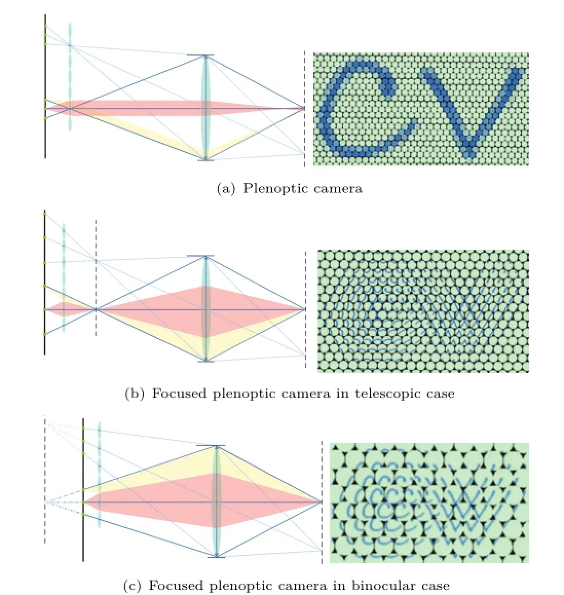
Fig.1　Different designs of light field camera and raw images that consist of many micro-lens images closely packed.

Decoding light field is equivalent to computing multiview images in two perpendicular directions. Multiview images are reorganized by selecting a contiguous set of pixels from each micro-lens image，for example，one pixel for plenoptic camera［2］and a patch for focused plenoptic camera［3，10］However，for a focused plenoptic camera，the patch size influences the focus depth of the rendered image. Such decoding method causes discontinuity on outof-focus area and results in artifact of aliasing.

For decoding a 2D raw image to a 4D light field representation，a common assumption is made that the center of each micro-lens image lies on the optical axis of its corresponding micro-lens［7，11，12］in ideal circumstances.Perwaß et al.［7］synthesized refocused images on different depths by searching pixels from multiple micro-lens images.Georgiev et al.［13］decoded into light field using ray transfer matrix analysis.Based on this assumption，the deviation in the ray's original direction has little effect on rendering a traditional image.However，the directions of decoded rays are crucial for an accurate estimation of camera intrinsic parameters，which is particularly important for absolute depth estimation ［14］or light field reparameterization for cameras in different poses［15］.

The calibration of a physical light field camera aimstodecoderaysmoreaccurately.Several methods are proposed for the plenoptic camera. Dansereauetal.［6］presenteda15-parameter plenoptic camera model to relate pixels to rays in 3D space，which provides theoretical support for light field panorama［15］.The parameters are initializedusingtraditionalcameracalibration techniques.Bok et al.［16］formulated a geometric projection model to estimate intrinsic and extrinsic parametersbyutilizingrawimagesdirectly，includinganalyticalsolutionandnon-linear optimization.Thomason et al.［17］concentrated on the misalignment of the micro-lens array and estimatedits positionandorientation.Inthis work，the directions of rays may deviate due to an inaccurate solution of the installation distances among main lens，micro-lens array，and image sensor.On the other hand，Johannsen et al.［12］estimated the intrinsic and extrinsic parametersfor a focused plenoptic camera by reconstructing a grid pattern from the raw image directly.The depth distortion caused by main lens was taken into account in their method.More importantly，expect for Ref.［17］，these methods do not consider the deviation of the image center or the optical center for each micro-lens，which tends to cause inaccuracy in decoded light field.

3　The world in camera

The distribution of rays refracted by a camera lens is different from the original light field.In this section，we first discuss the corresponding relationship between the points in the scene and inside the camera modelled as a thin lens.Then we analyze the invariance in an ideal focused plenoptic camera，based on a thin lens and a pinhole model forthemainlensandmicro-lensrespectively. Finally we conclude the relationship between the raw image features and the depth-scale information in the scene.Our analysis is conducted in the non-homogeneous coordinate system.

3.1Thin lens model

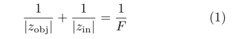
As shown in Fig.2，the rays emitted from the scene point（xobj，yobj，zobj）Tin different directions are refracted through the lens aperture and brought to a single convergence point（xin，yin，zin）Tif zobj＞F，where F denotes the focal length of the thin lens. The relationship between the two points is described as follows:

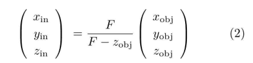
Equation（2）showsthattheratioonthe coordinates of the two points changes with zobj. Furthermore，thereisaprojectiverelationship between the coordinates inside and outside the camera.For example，as shown in Fig.3，the objects with the same size in different depths in the scene correspond to the objects with different sizes inside the camera.The relationship can be described as

where the focal length F satisfies:

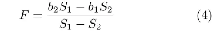
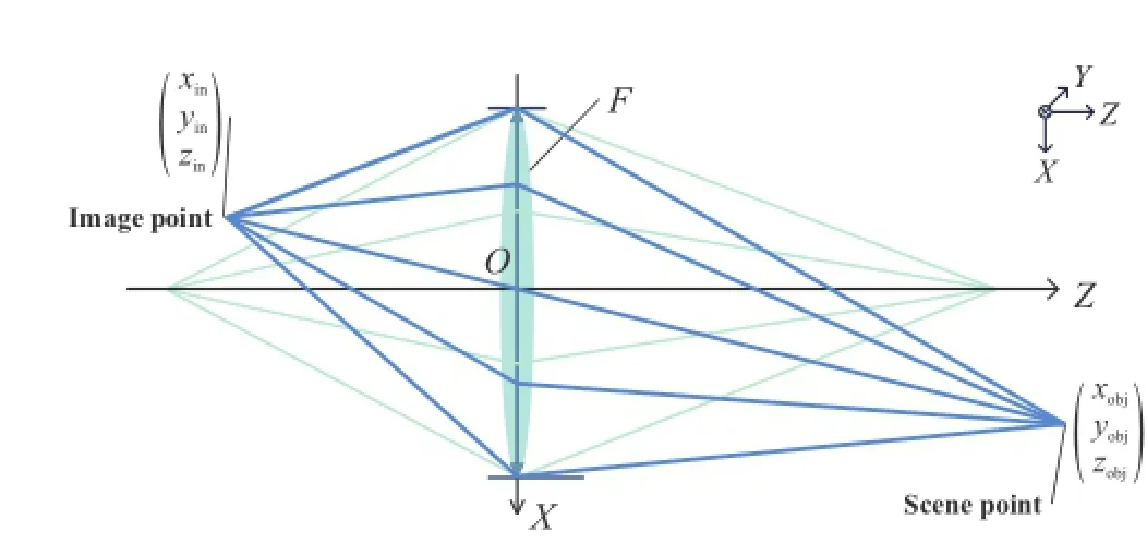
Fig.2　Thin lens model.

3.2Ideal focused plenoptic camera model

As shown in Fig.1，there are two optical designs of the focused cameras.In this paper，we only consider the design in Fig.1（b）.The case in Fig.1（c）is similar to the former，only with the difference in the relative position of the focus point and the optical center of the micro-lens.

In this section，the main lens and the micro-lens array are described by a thin lens and a pinhole model respectively.As shown in Fig.4，the main lens，the micro-lens array，and the image sensor are parallel to each other and all perpendicular to the optical axis.The optical center of the main lens lies on the optical axis.

Let dimgand dlensbe the distance between two geometric centers of arbitrary adjacent microlens images and the diameter of the micro-lens respectively，as shown in Fig.4（a）.The ratio between them is

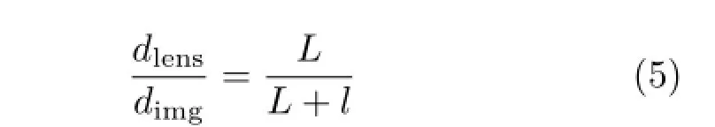
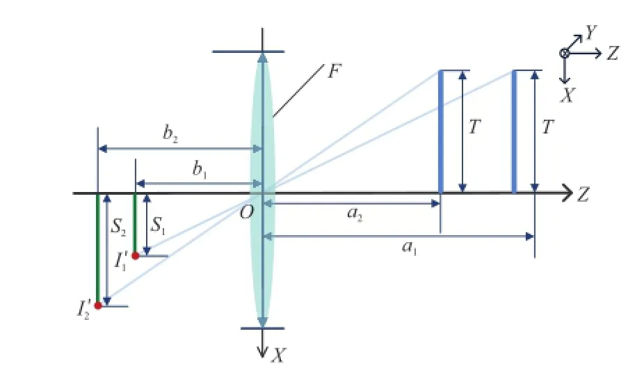
Fig.3　Two objects with the same size of T in the scene at different depths focus inside a camera with focal length F.

where L and l are the distances among the main lens，the micro-lens array，and the image sensor respectively.We can find that the ratio L/l is

dependent on the raw image and the diameter of micro-lens，which is useful for our calibration model in Section 5.Moreover，there is a deviation between the optical center of micro-lens and the geometric center of its image，and dimgis constant in the same plenoptic camera.

Let dlens，sceneand dimg，scenebe the size of microlens and its image refracted through the main lens into the scene respectively（Fig.4（b）），combining Eqs.（2）and（5），the ratio between them satisfies:

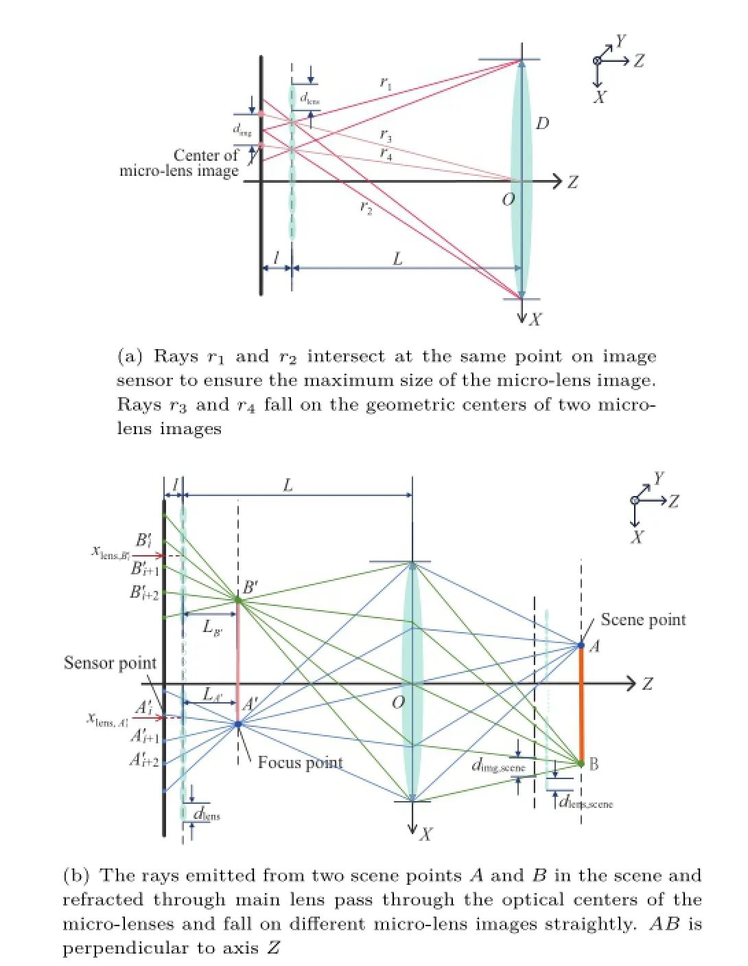
Fig.4　Ideal focused plenoptic camera in telescopic case.

Equation（6）shows that though the rays are refracted through the main lens，the deviation between the geometric center of micro-lens image and the optical center of micro-lens still can not be ignored.The effect of deviations on the rendered imageswill bedemonstrated and discussedin experiment.

In Fig.4（b），A′and B′are the focus points of two scene points A and B respectively.The rays emitted from every focus point fall on multiple micro-lens and focus on the image sensor，resulting in multiple images A′iand Bi′.The distance between sensor

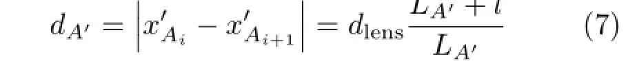
where LA′is the distance between focus point A′and the micro-lens array，and|·|denotes the absolute operator.Equation（7）indicates that the distance between arbitrary two adjacent sensor points of the same focus point inside the camera is only dependent on intrinsic parameters.Once the raw image is shot （thus dA′is determined），LA′is only dependent on l and dlens.According to triangle similarity，we can get the coordinate of the focus point:

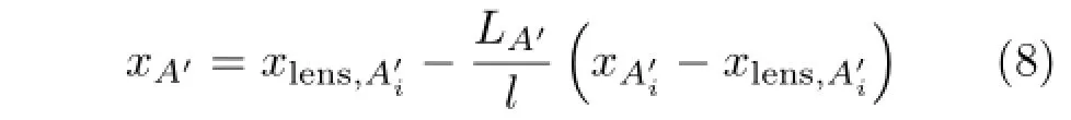
Based on Eq.（7），we can simplify Eq.（8）as

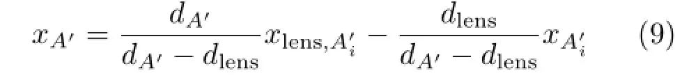
According to Eq.（9），once a raw image is shot（thusandare determined）andis given，xA′and yA′can be calculated and they areindependentonotherintrinsicparameters. Furthermore，the length of AB can be calculated using only the raw image and dlens.

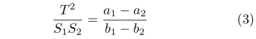
Imaging that there are two objects with equal size in the scene，as shown in Fig.3，the distance between the focus point and the micro-lens array can be calculated via Eq.（7）.Replacing b1and b2in Eq. （4）and simplifying via Eqs.（5）and（7），we get the relationship:

where S1，S2，LI′1，and LI′2are dependent on only three factors，including the raw image，dlens，and l.Equation（10）shows that the value of F can be calculated uniquely once the other intrinsic parameters are determined.

In the same manner，Eq.（3）can be simplified as

From Eq.（11），the size of an object in the scene is independent on l.The size of an object which we reconstruct from the raw image can not be taken as a cost function to constrain l.

In summary，given the coordinates of micro-lens and the raw image，three theorems can be concluded as follows:

（1）The size of a reconstructed object inside the camera and its distance to the micro-lens array are constant（Eq.（9））.

（2）The unique F can be determined by the prior of the scene（Eq.（10））.

（3）The size of the reconstructed object in the scene is constant with changing L（Eq.（11））.

4　Micro-lens-based camera model

In this section we present a more complete model for a focused plenoptic camera with misalignment of the micro-lens array［17］，which is capable of decoding more accurate light field.There are 10 intrinsic parameters totally to be presented in this section，including the distance between the main lens and the micro-lens array，L，the distance between the micro-lens array and the image sensor，l，the misalignment of micro-lens array，xm，ym，（θ，β，γ），the focal length of the main lens，F，and the shift of image coordinate，（u0，v0）.

4.1Distribution of micro-lens image

As shown in Fig.5（a），every micro-lens with its unique coordinate（xi，yi，0）Tis tangent with each other.In addition，（xi，yi，0）Tis only dependent on dlens.To simplify the discussion，we assume the layout of the micro-lens array is square-like.For hexagon-like configuration，it is easy to partition the whole array into two square-like ones.With the transformation shown in Fig.5（b），the coordinate of the optical center of the micro-lens is represented as

where t=（xm，ym，L）Tand R is the rotation matrix with three degrees of freedom，i.e.，the rotations （θ，β，γ）about three coordinate axes，which are similar to the traditional camera calibration model ［18］.

Although the main lens and the image sensor are parallel，the case between the micro-lens array and the image sensor is not similar（Fig.5（c））. Each geometric center of the micro-lens image is represented as

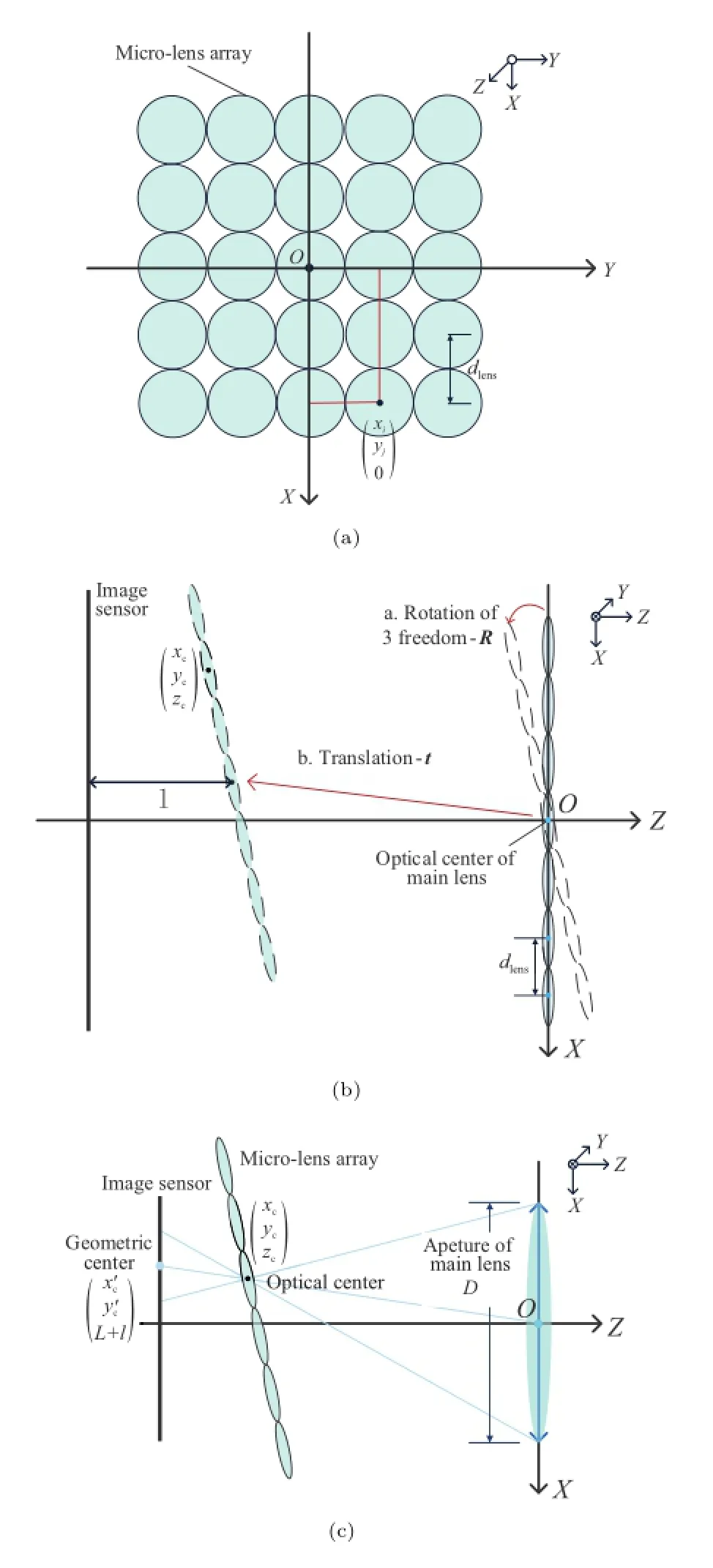
Fig.5　The coordinate system of a focused plenoptic camera.

4.2Projections from the raw image

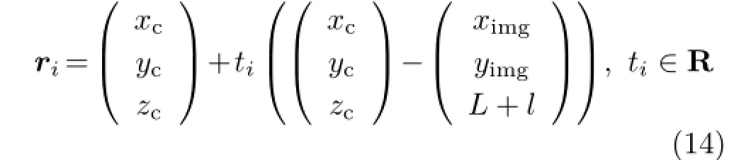
Once the coordinate of a micro-lens's optical center （xc，yc，xc）Tand its image point（ximg，yimg，L+l）Tare calculated，we can get a unique ray rirepresented as

As shown in Fig.4（b），the multiple imageson the image sensor from the same focus point A′can be located if a proper pattern is shot，such as a grid-array pattern［12］. Thus the multiple rays emitted from point A′through different optical centers of the micro-lenses are collected to calculate the coordinate of point A′:

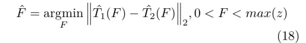
where‖·‖2represents L2norm.Till now，we have accomplished the decoding process of light field inside the camera.To obtain the light field data in the scene，combining the depth-dependent scaling ratio described in Eq.（2），the representation of the focused pointsˆA′can be transformed using the focal lens F easily.

5　Calibration

Compared to the ideal focused plenoptic camera model，the shift caused by the rotations of related micro-lenses is far less than l and the difference in the numerical calculation is trivial，therefore the three theorems concluded for an ideal focused plenoptic camera still hold for our proposed model with misalignment.More importantly，when there iszeromachiningerror，thediameterofthe micro-lens dlensis set，and does not need to be estimatedduringthecalibration.Consequently，the unique solution of the intrinsic parameters PPP=（θ，β，γ，xm，ym，L，l，u0，v0）TandFcanbe estimated using the two steps described in the following.

5.1Decoding by micro-lens optical center

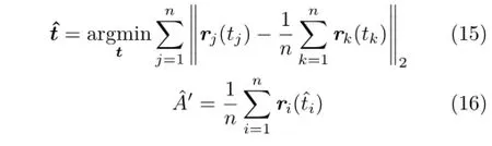
To locate the centers of the micro-lens images，we shoot a white scene［19，20］.Then a template of proper size is cut out from the white image and its similarity with the original white image is calculated via normalized cross-correlation（NCC）.To find the locations with subpixel accuracy，a threshold is placed on the similarity map such that all values less than 50%of the maximum intensity are set to zero. Then we take the filtered similarity map as weight and calculate the weighted coordinate of every small region.The results are shown in Fig.6.

Fig.6　The template（top-left），the crops of similarity map（topright），the filtered similarity map（bottom-left），and the final location of the micro-lens image centers（bottom-right）.

To estimate parametersPPP，we minimize the cost function:

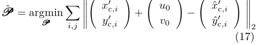
where（u0，v0）is the offset between the camera coordinate and the image coordinate.After this optimization，PPPis used to calculate micro-lens opticalcentersandreconstructthecalibration points.Then the rays are obtained via Eq.（14）.

According to Eq.（5），the solution of Eq.（17），changing with the initial value of L，is not unique. Moreover，the ratio L/l is almost constant with changing initial value ofPPP.Although there are differences between the models described in Section 3.2 and Section 4，the theorems still hold since the shift caused by the rotations can be ignored.This observation will be verified in experiment later.

In addition，the value of l influences the direction of decoded rays.Due to the coupling relationship of angle and depth，either of them can be used as the prior to be introduced to estimate the uniquePPP.

5.2Reconstruction of calibration points To reconstruct a plane in the scene，we may shoot a certain pattern in order to recognize multiple images from different scene points.A crop of the calibration board and its raw image we shoot are shown in Fig.7. To locate the multiple images of every point on the calibration board，we preprocess the grid image by adding the inverse color of the white image to the grid image（Fig.7）.Then one of the sensor points corresponding to the focus point A′，denoted byis located by the same method described in Section 5.1.Consequently，the plane we shoot in the scene，denoted byˆΠ=｛Ai|i=1，···，n｝，is easy to be reconstructed using Eqs.（2）and（14）.

As shown in Fig.8，we design a parallel biplanar board with known distance between the two parallel planes and the distance between adjacent grids，which can provide depth prior Prdpand scale prior Prsc.Equivalently，we can shoot a single-plane board twice while we move the camera on a guide rail to a fixed distance.

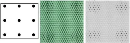
Fig.7　A crop of calibration board，its raw image，and the preprocessed image by white image.

Note that if the values of L or l is incorrect，the distance between planeandis not equal to the prior distance.Therefore we take the distance

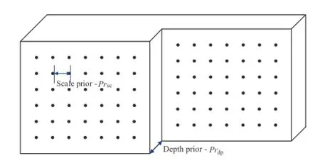
Fig.8　The parallel biplanar board we designed to provide depth prior for calibration.

where dis（·，·）represents the distance between two parallel planes.In practice，we take the mean distance of reconstructed points onˆΠ1to planeˆΠ2as the value of dis.

Moreover，ˆT1andˆT2may not be equal to Prscdue to possible calculation error，so we must refine the value of depth prior to ensure the correct ratio of scale and depth.

5.3Algorithm summary

Thecompletealgorithmissummarizedin Algorithm 1.

To make the algorithm more efficiently，the searchstep of the loop of L should be changed with the value of‖dis）-Prdp‖2in Eq.（19）. The same principle is applied to the search step of F.In addition，because of the monotonicity of‖dis）-Prdp‖2with L，and Fwith，we can use dichotomy to search an accurate value more efficiently.

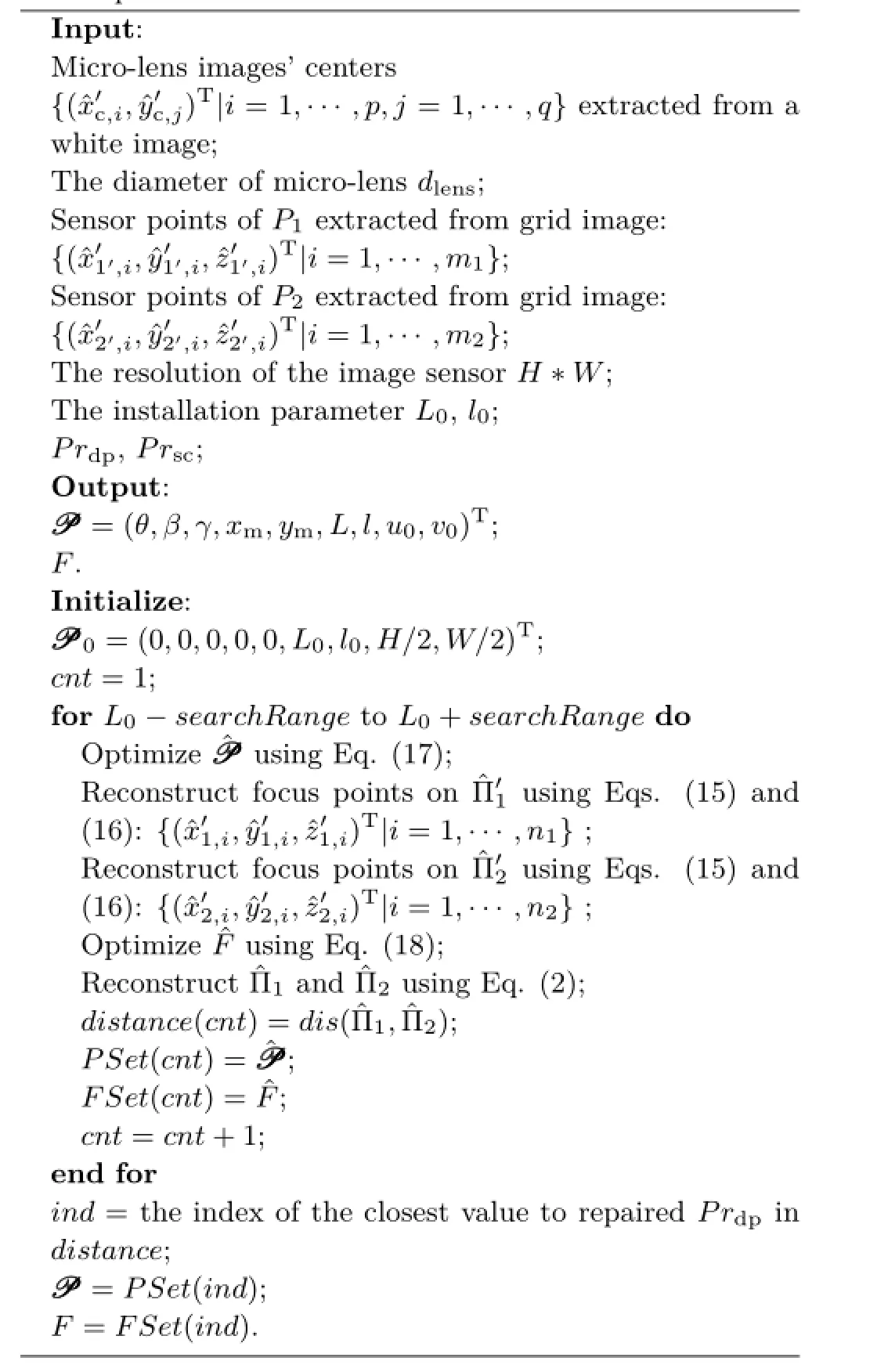
Algorithm 1:Calibration method for a focused camera with a parallel calibration board

6　Experimental results

In experiments，we apply our calibration method on simulated and real world scene data.We capture three datasets of white images and grid images using a self-assembly focused plenoptic camera（Fig.9）. The camera includes a GigE camera with a CCD image sensor whose resolution is 4008×2672 pixels that are 9μm wide，F-mount Nikon lens with 50mm focal length，and a micro-lens array whose diameter is 300μm with negligible error in hexagon layout.

We use the function“fminunc”in MATLAB to complete the non-linear optimization in Eqs.（15），（17），and（18）.The initial parameters are set as the installation parameters，and θ，β，γ，xm，ymare set to zero.

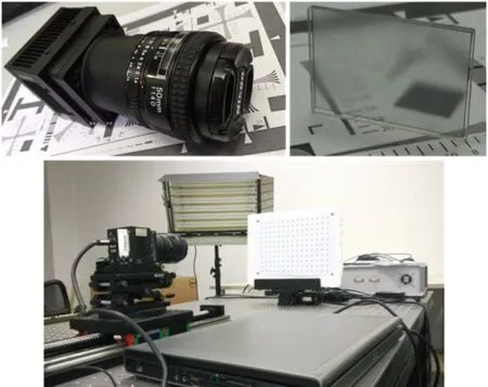
Fig.9　The focused plenoptic camera we installed and its micro-lens array inside the camera.

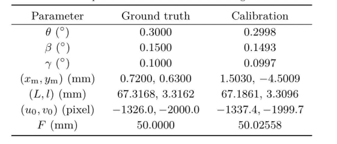
Table 1　The parameters we estimated and the ground truth

6.1Simulated data

First we verify the calibration method on simulated images rendered in MATLAB，as shown in Fig.1. The ground truth and the calibrated parameters are shown in Table 1.We compare the estimated angle of the ray passing through each optical center of microlens and the one of the main lens to the ground truth，which is shown in Fig.10.The differences are less than 1.992×10-3rad.

We compare the geometric centers of the microlens images we locate and the ones with optimization. Theerrormapsof84×107geometriccenters optimized with different L are shown in Fig.11（a）. From Fig.11（b），we find that there are 96.53%of the centers whose error is less than 0.1 pixel，which is the input for the following projection step.

The comparison of the locations of optical centers of micro-lenses with different L is illustrated in Fig.12.Thedifferenceinx-coordinateandycoordinate of the optical center is trivial with changing L.The maximal difference is 4.2282× 10-6mm when L changes from 55 to 84mm，which proves our observation mentioned in Section 5.1.

Fig.10 The histogram of the deviation between the estimated angles of the rays and the ground truth.

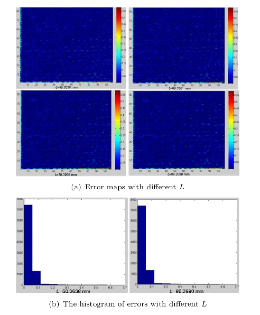
Fig.11　The results of optimization on geometric centers of the micro-lens image on simulated data.

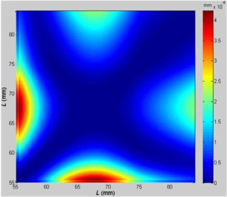
Fig.12　The comparison of the locations of optical centers of microlenses with different L from 55 to 84mm on simulated data.The value in row i and column j represents the difference in x-coordinate and y-coordinate between the results optimized in Liand Lj.

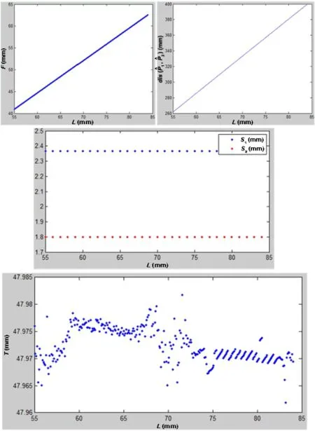
Fig.13　The values of F，dis（ˆΠ1，ˆΠ2），ˆS1，ˆS2，andˆT（ˆT2= ˆT1）with different L on simulated data.

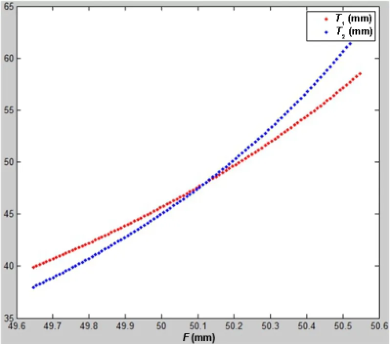
Fig.14　The relationship ofˆT1，ˆT2，and F when L=67.3129mm.

6.2Physical camera

Then we verify the calibration method on the physical focused plenoptic camera.To obtain the equivalent data of parallel biplanar board，we shoot a single-plane board twice while we move the camera on a guide rail to an accurate fixed distance，as shown in Fig.9.The depth prior Prdpis precisely controlled to be 80.80mm and the scale prior Prscis 28.57mm.The calibration results are shown in Fig.15.

As shown in Fig.15（a），there is an obvious error between the computed geometric centers and the located centers on the edge of the error map，which may result from the distortion of lenses or the machining error of micro-lens.However，we find that that there are 73.00%of the centers whose error is less than 0.6 pixel，as shown in Fig.15（b）.Themean difference of geometric centers of micro-lens images optimized with different L is 1.89×10-4pixel （Fig.15（c））.The results of F，dis（ˆΠ1，ˆΠ2），ˆS1，ˆS2，ˆT （ˆT1= ˆT2）with different L are similar to the results on simulated data.

Finally，to verify the stability of our algorithm，we calibrate intrinsic parameters with different poses of calibration board.Corresponding results are shown in Table 2.

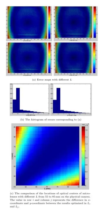
Fig.15　The results of optimization on geometric centers of microlens image on physical data.

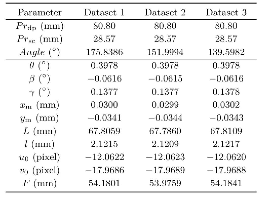
Table 2　Parameters estimated with calibration board with different poses.The third parameter is the angle between the calibration board and the optical axis

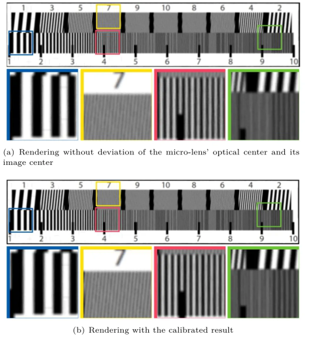
Fig.16　The rendered images from simulated data.

6.3Rendering

Werenderthefocusedimagewithdeviations between the optical center of micro-lens and the geometric center of micro-lens image.

We shoot a resolution test chart on the same depth for simulated data（Fig.16），which indicates that the deviation surely effects the accuracy of decoded lightfield.Then we shoot a chess board for simulated data to evaluate the width of every grid in the rendered images.We resize the images by setting the mean width of the grids to be 100pixels.Then we calculate the range and the standard deviation of the grid width.The results are shown in Table 3，which indicates that the calibration contributes to the uniform scale in the same depth and reduces the distortion caused by incorrect deviations.The results on physical camera are shown in Table 4 and Fig.17.The decoded light field with the estimated intrinsic parameters leads to more accurate refocus distance［14］，which is equivalent to a correct ratio of scale and depth.

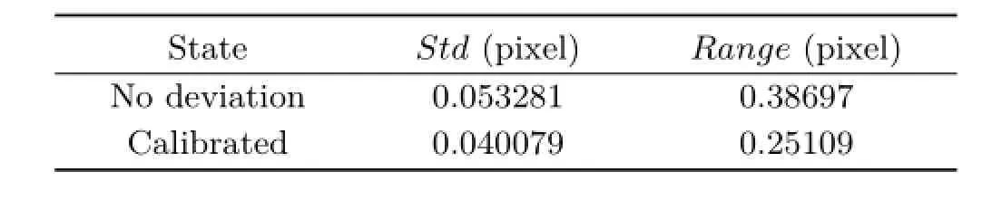
Table 3　The range and variance of rendered chess board on simulated data

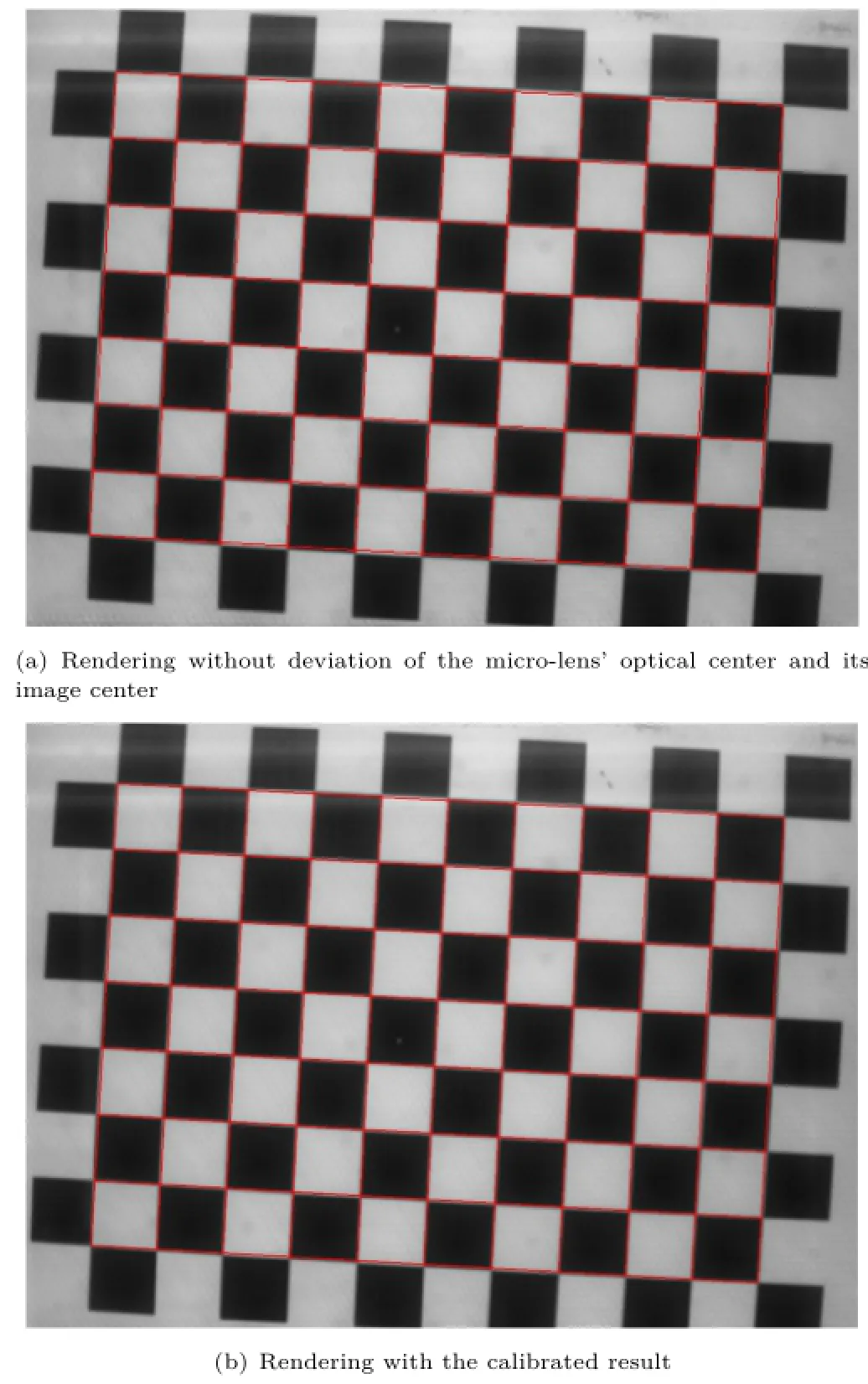
Fig.17　The image rendered from physical camera.

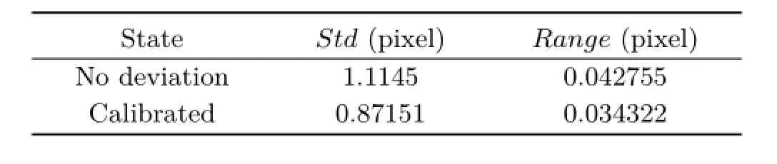
Table 4　The range and variance of rendered chess board on physical camera

7　Conclusions and future work

In the paper we present a 10-intrinsic-parameter model to describe a focused plenoptic camera with misalignment.To estimate the intrinsic parameters，we propose a calibration method based on the relationship between the raw image features and the depth-scale information in the real world scene.To provide depth and scale priors to constrain the intrinsic parameters，we design a parallel biplanar boardwithgrids.Thecalibrationapproachis evaluatedonsimulationaswellasrealdata. Experimental results show that our proposed method is capable of decoding more accurate light field for the focused plenoptic camera.

Future work includes modelling the distortion caused by the micro-lens and main lens，optimization of extrinsic parameters，and the reparameterization of multiple and re-sampling light field data from cameras with different poses.

Acknowledgements

The work is supported by the National Natural Science Foundation of China（Nos.61272287 and 61531014）and the research grant of State Key LaboratoryofVirtualRealityTechnologyand Systems（No.BUAAVR-15KF-10）.

References

［1］Ng，R.Digital light field photography.Ph.D.Thesis. Stanford University，2006.

［2］Ng，R.；Levoy，M.；Bredif，M.；Duval，G.；Horowitz，M.；Hanrahan，P.Light field photography with a handheld plenoptic camera.Stanford University Computer Science Tech Report CSTR 2005-02，2005.

［3］Georgiev，T.G.；Lumsdaine，A.Focused plenoptic camera and rendering.Journal of Electronic Imaging Vol.19，No.2，021106，2010.

［4］Lumsdaine，A.；Georgiev，T.Full resolution lightfield rendering.Technical Report.Indiana University and Adobe Systems，2008.

［5］Lumsdaine，A.；Georgiev，T.The focused plenoptic camera.In:ProceedingsofIEEEInternational Conference on Computational Photography，1-8，2009.

［6］Dansereau，D.G.；Pizarro，O.；Williams，S.B. Decoding，calibration and rectification for lenseletbasedplenopticcameras.In:Proceedingsof IEEE Conference on Computer Vision and Pattern Recognition，1027-1034，2013.

［7］Perwaß，C.；Wietzke，L.Single lens 3D-camera with extended depth-of-field.In:Proceedings of SPIE 8291，Human Vision and Electronic Imaging XVII，829108，2012.

［8］Bishop，T.E.；Favaro，P.Plenoptic depth estimation from multiple aliased views.In:Proceedings of IEEE 12th International Conference on Computer Vision Workshops，1622-1629，2009.

［9］Levoy，M.；Hanrahan，P.Lightfieldrendering. In:Proceedings of the 23rd Annual Conference on Computer Graphics and Interactive Techniques，31-42，1996.

［10］Wanner，S.；Fehr，J.；J¨ahne，B.Generating EPI representations of 4D light fields with a single lens focusedplenopticcamera.In:Lecture Notes in Computer Science，Vol.6938.Bebis，G.；Boyle，R.；Parvin，B.et al.Eds.Springer Berlin Heidelberg，90-101，2011.

［11］Hahne，C.；Aggoun，A.；Haxha，S.；Velisavljevic，V.；Fern´andez，J.C.J.Light field geometry of a standard plenoptic camera.Optics Express Vol.22，No.22，26659-26673，2014.

［12］Johannsen，O.；Heinze，C.；Goldluecke，B.；Perwaß，C.On the calibration of focused plenoptic cameras. In:Lecture Notes in Computer Science，Vol.8200. Grzegorzek，M.；Theobalt，C.；Koch，R.；Kolb，A.Eds. Springer Berlin Heidelberg，302-317，2013.

［13］Georgiev，T.；Lumsdaine，A.；Goma，S.Plenoptic principal planes.Imaging Systems and Applications，OSA Technical Digest（CD），paper JTuD3，2011.

［14］Hahne，C.；Aggoun，A.；Velisavljevic，V.The refocusingdistanceofastandardplenoptic photograph.In:Proceedings of 3DTV-Conference: The True Vision—Capture，Transmission and Display of 3D Video，1-4，2015.

［15］Birklbauer，C.；Bimber，O.Panorama light-field imaging.Computer Graphics Forum Vol.33，No.2，43-52，2014.

［16］Bok，Y.；Jeon，H.-G.；Kweon，I.S.Geometric calibrationofmicro-lens-basedlight-fieldcameras using line features.In:Lecture Notes in Computer Science，Vol.8694.Fleet，D.；Pajdla，T.；Schiele，B.；Tuytelaars，T.Eds.Springer International Publishing，47-61，2014.

［17］Thomason，C.M.；Thurow，B.S.；Fahringer，T. W.Calibration of a microlens array for a plenoptic camera.In:Proceedings of the 52nd Aerospace Sciences Meeting，AIAA SciTech，AIAA 2014-0396，2014.

［18］Zhang，Z.Aflexiblenewtechniqueforcamera calibration.IEEE Transactions on Pattern Analysis and Machine Intelligence Vol.22，No.11，1330-1334，2000.

［19］Cho，D.；Lee，M.；Kim，S.；Tai，Y.-W.Modeling the calibration pipeline of the Lytro camera for highqualitylight-fieldimagereconstruction.In: Proceedings of IEEE International Conference on Computer Vision，3280-3287，2013.

［20］Sabater，N.；Drazic，V.；Seifi，M.；Sandri，G.；Perez，P.Light-field demultiplexing and disparity estimation.2014.Available at https://hal.archivesouvertes.fr/hal-00925652/document.

Chunping Zhang received her B.E. degreefromSchoolofComputer Science， NorthwesternPolytechnical Universityin2014.Sheisnowa M.D.student at School of Computer Science， NorthwesternPolytechnical University.Herresearchinterests includecomputationalphotography，and light field computing theory and application.

Zhe Ji received her B.E.degree in technology and computer science from Northwestern Ploytechnical University in 2015.She is now a M.D.student atSchoolofComputerScience，Northwestern Polytechnical University. Hercurrentresearchinterestsare computational photography，and light field computing theory and application.

Qing Wang is now a professor and Ph.D.tutor at School of Computer Science， NorthwesternPolytechnical University.Hegraduatedfromthe DepartmentofMathematics，Peking Universityin1991.Hethenjoined Northwestern Polytechnical University as a lecturer.In 1997 and 2000，he obtained his master and Ph.D.degrees from the Department ofComputerScienceandEngineering，Northwestern Polytechnical University，respectively.In 2006，he was awarded the Program for New Century Excellent Talents in University of Ministry of Education，China.He is now a member of IEEE and ACM.He is also a senior member of China Computer Federation（CCF）.

He worked as research assistant and research scientist in the Department of Electronic and Information Engineering，the Hong Kong Polytechnic University from 1999 to 2002.He also worked as a visiting scholar at the School of Information Engineering，the University of Sydney，Australia，in 2003 and 2004.In 2009 and 2012，he visited the Human Computer Interaction Institute，Carnegie MellonUniversity，for six months and the Department of Computer Science，University of Delaware，for one month，respectively.

Professor Wang's research interests include computer visionandcomputationalphotography，suchas3D structureandshapereconstruction，objectdetection，tracking and recognition in dynamic environment，and light field imaging and processing.He has published more than 100 papers in the international journals and conferences.

Open AccessThe articles published in this journal aredistributedunderthetermsoftheCreative Commons Attribution 4.0 International License（http:// creativecommons.org/licenses/by/4.0/）， whichpermits unrestricted use，distribution，and reproduction in any medium，provided you give appropriate credit to the original author（s）and the source，provide a link to the Creative Commons license，and indicate if changes were made.

Other papers from this open access journal are available free of charge from http://www.springer.com/journal/41095. To submit a manuscript，please go to https://www. editorialmanager.com/cvmj.

Xiaole Zhao1（），Yadong Wu1，Jinsha Tian1，and Hongying Zhang2
○cThe Author（s）2016.This article is published with open access at Springerlink.com

AbstractIt has been widely acknowledged that learning-basedsuper-resolution（SR）methodsare effective to recover a high resolution（HR）image from a single low resolution（LR）input image.However，there exist two main challenges in learning-based SR methods currently:the quality of training samples and the demand for computation.We proposed a novel framework for single image SR tasks aiming at these issues，which consists of blind blurring kernel estimation（BKE）and SR recovery with anchored space mapping（ASM）.BKE is realized via minimizing the cross-scale dissimilarity of the image iteratively，and SR recovery with ASM is performed based on iterative least square dictionary learning algorithm（ILS-DLA）.BKE is capable of improving the compatibility of training samples and testing samples effectively and ASM can reduce consumed time during SR recovery radically. Moreover，a selective patch processing（SPP）strategy measured by average gradient amplitude|grad|of a patch is adopted to accelerate the BKE process.The experimental results show that our method outruns several typical blind and non-blind algorithms on equal conditions.

Keywordssuper-resolution（SR）；blurring kernel estimation（BKE）； anchoredspace mapping（ASM）；dictionary learning；average gradient amplitude

1School of Computer Science and Technology，Southwest University of Science and Technology，Mianyang 621010，China.E-mail:X.Zhao，zxlation@foxmail.com（）；Y. Wu，wyd028@163.com.

2School of Information Engineering，Southwest University of Science and Technology，Mianyang 621010，China.E-mail:zhy0838@163.com.

Manuscript received:2015-11-20；accepted:2016-02-02

1　Introduction

Single image super-resolution has been becoming the hotspot of super-resolution area for digital images because it generally is not easy to obtain an adequate number of LR observations for SR recovery in many practical applications.In order to improve image SR performance and reduce time consumption so that it can be applied in practical applications more effectively，this kind of technology has attracted great attentions in recent years.

Singleimagesuper-resolutionisessentiallya severe ill-posed problem，which needs adequate priorstobesolved.Existingsuper-resolution technologies can be roughly divided into three categories:traditionalinterpolationmethods，reconstruction methods，and machine-learning（ML）basedmethods.Interpolationmethodsusually assume that image data is continuous and bandlimited smooth signal.However，there are many discontinuousfeaturesinnaturalimagessuch as edges and corners etc.，which usually makes the recovered images by traditional interpolation methods suffer from low quality［1］.Reconstruction based methods apply a certain prior knowledge，such as total variation（TV）prior［2-4］and gradient profile（GP）prior［5］etc.，to well pose the SR problem.The reconstructed image is required to be consistent with LR input via back-projection.But a certain prior is typically only propitious to specific images.Besides，these methods will produce worse results with larger magnification factor.

Relativelyspeaking， machine-learningbased method is a promising technology and it has become the most popular topic in single image SR field. The first ML method was proposed by Freemanet al.［6］，which is called example-based learning method.This method predicts HR patches from LR patches by solving markov random field（MRF）model by belief propagation algorithm.Then，Sun et al.［7］enhanced discontinuous features（such as edges and corners etc.） by primal sketch priors. These methods need an external database which consists of abundant HR/LR patch pairs，and time consumption hinders the application of this kind of methods.Chang et al.［8］proposed a nearest neighbor embedding（NNE）method motivated by the philosophy of locally linear embedding（LLE）［9］.They assumed LR patches and HR patches have similar space structure，and LR patch coefficients can be solved through least square problem for the fixed number of nearest neighbors（NNs）.These coefficients are then used for HR patch NNs directly. However，the fixed number of NNs could cause over-fitting and/or under-fitting phenomena easily ［10］.Yang et al.［11］proposed an effective sparse representation approach and addressed the fitting problems through selecting the number of NNs adaptively.

However，ML methods are still exposed to two main issues:the compatibility between training and testing samples（caused by light condition，defocus，noise etc.），and the mapping relation between LR and HR feature spaces（requiring numerous calculations）.Glasner et al.［12］exploited image patch non-local self-similarity（i.e.，patch recurrence）within image scale and cross-scale for single image SR tasks，which makes an effective solution for the compatibility problem.The mapping relation involves the learning process of LR/HR dictionaries. Actually，LR and HR feature spaces are tied by some mapping function，which could be unknown and not necessarily linear［13］.Therefore，the originally direct mapping mode［11］may not reflect this unknown non-linear relation correctly.Yang et al.［14］proposed another joint dictionary training approach to learn the duality relation between LR/HRpatchspaces.Themethodessentially concatenates the two feature spaces and converts the problem to the standard sparse representation. Further，they explicitly learned the sparse coding problem across different feature spaces in Ref.［13］，whichisso-calledcoupleddictionarylearning （CDL）algorithm.He et al.［15］proposed another beta process joint dictionary learning（BPJDL）for CDL based on a Bayesian method through using a beta process prior.But，above-mentioned dictionary learning approaches did not take the feature of training samples into account for better performance.Actually，it is not an easy work to find the complicated relation between LR and HR feature spaces directly.

We present a novel single image super-resolution methodconsideringbothSRresultandthe acceleration of execution in the paper.The proposed approach firstly estimated the true blur kernel based on the philosophy of minimizing the dissimilarity between cross-scale patches［16］.LR/HR dictionaries then were trained via input image itself downsampled by the estimated blur kernel.The BKE processing was adopted for improving the quality of training samples.Then，L2norm regularization was used to substitute L0/L1norm constraint so that latent HR patch can be mapped on LR patch directly through a mapping matrix computed by LR/HR dictionaries.This strategy is similar with ANR［17］，but we employed a different dictionary learning approach，i.e.，ILS-DLA，to train LR/HR dictionaries.In fact，ILS-DLA unified the principle ofoptimizationofthewholeSRprocessand produced better results with regard to K-SVD used by ANR.

The remainder of the paper is organized as follows: Section 2 briefly reviews the related work about this paper.The proposed approach is described in Section 3 detailedly.Section 4 presents the experimental results and comparison with other typical blind and non-blind SR methods.Section 5 concludes the paper.

2　Related work

2.1Internal statistics in natural images

Glasner et al.［12］exploited an important internal statistical attributes of natural image patches named the patch recurrence，which is also known as image patch redundancy or non-local self-similarity （NLSS）.NLSS has been employed in a lot of computer vision fields such as super resolution［12，18-21］，denoising［22］，deblurring［23］，and inpainting ［24］etc.Further，Zontak and Irani［18］quantified this property by relating it to the spatial distance from

the patch and the mean gradient magnitude|grad|of a patch.The three main conclusions can be perceived according to Ref.［18］:（i）smooth patches recur very frequently，whereas highly structured patches recur much less frequently；（ii）a small patch tends to recur densely in its vicinity and the frequency of recurrence decays rapidly as the distance from the patch increases；（iii）patches of different gradient content need to search for nearest neighbors at different distances.These conclusions consist of the theoretical basis of using the mean gradient magnitude|grad|as the metric of discriminatively choosing different patches when estimating the blurring kernels.

2.2Cross-scale blur kernel estimation

For more detailed elaboration，we still need to briefly review the cross-scale BKE and introduce our previous work［16］on this issue despite a part of it is the same as previous one.We will illustrate the detailed differences in Section 3.1.Because of camera shake，defocus，and various kinds of noises，the blur kernel of different images may be entirely and totally different.Michaeli and Irani［25］utilized the non-local self-similarity property to estimate the optimal blur kernel by maximizing the crossscale patch redundancy iteratively depending on the observation that HR images possess more patch recurrence than LR images.They assumed the initial kernel is a delta function used to down-sample the input image.A few NNs of each small patch were found in the down-sampled version of input image. Each NN corresponds to a large patch in the original scale image，and these patch pairs construct a set of linear equations which could be solved by using weighted least squares.The root mean squared error （RMSE）between cross-scale patches was employed as the iteration criterion.Figure 1 shows the main process of cross BKE of Ref.［25］.We follow the same idea with more careful observation:the effect of the convolution on smooth patches is obviously smaller than that on structured patches（refer to Fig.2）. This phenomenon can be explained easily according to the definition of convolution.Moreover，the mean gradient magnitude|grad|is more expressive than the variance of a patch on the basis of the conclusions in Ref.［18］.

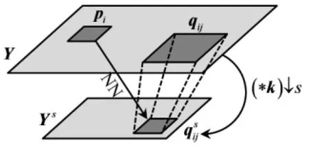
Fig.1　Description of cross-scale patch redundancy.For each small patch piin Y，finding its NNsinwhich corresponds to a large patch qijin Y，andconstitute a patch pair，and all patch pairs of NNs construct a set of linear equations which is solved using weighted least squares to obtain an updated kernel.

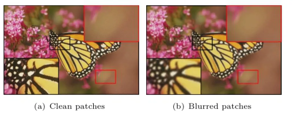
Fig.2　Blurring effect on non-smooth and smooth areas.Black boxes indicate structured areas，and red boxes indicate smooth areas. （a）Clean patches.It can be clearly seen that the structure of nonsmooth patch is distinct.（b）Blurred patches corresponding to（a）. The detail of non-smooth patch is obviously blurry.

2.3ILS-DLA and ANR

ILS-DLA is a typical dictionary learning method. It adopts an overall optimization strategy based on least square（LS）to update the dictionary when the weight matrix is fixed so that ILS-DLA［26］is usually faster than K-SVD［17，27］.Besides，ANR just adjusts the objective function slightly and the SR reconstruction process is theoretically based on least square method.

Supposing we have two coupled feature sets FLand FHwith size nL×L and nH×L，and the number of the atoms in LR dictionary DLand HR dictionary DHis K.The training process for DLcan be described as

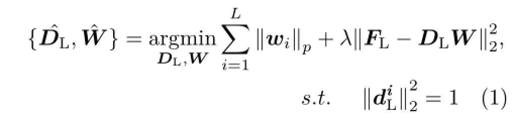
where diLis an atom in DL，wiis a column vector in W.p∈｛0，1｝is the constrain of the coefficient vector wi，and λ is a tradeoff parameter.Equation （1）is usually resolved by optimizing one variable while keeping the other one fixed.In ILS-DLA case，least square method is used to update DLwhile W is fixed.Once DLand W were obtained then we couldcompute the DHaccording to the same LS rule:

According to the philosophy of ANR，a mapping matrix can be calculated through the weight matrix and the both dictionaries.Then，it is used to project LR feature patches to HR feature patches directly. Thus，L0/L1norm constrained optimization problem degenerates to an issue of matrix multiplication.

3　Proposed approach

3.1Improved blur kernel estimation

Referring to Fig.1，we use Y to represent the input LR image，and X to be latent HR image.Michaeli and Irani［25］estimated the blur kernel through maximizing the cross-scale NLSS directly，while we minimized the dissimilarity between cross-scale patches.Despite these two ideas look like the same with each other intuitively，they are slightly different and lead to severely different performance［16］.While Ref.［16］has introduced this part of content in detail，we need to present the key component of the improved blur kernel estimation for integrated elaboration.The following objective function has reflected the idea of minimizing the dissimilarity between cross-scale patches:

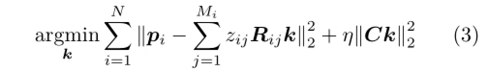
whereNisthenumberofquerypatchesin Y.Matrix Rijcorresponds to the operation of convolving with qijand down-sampling by s.C is a matrix used as the penalty of non-smooth kernel. The second term of Eq.（3）is kernel prior and η is the balance parameter as the tradeoff between the error term and kernel prior.For the calculation of the weight zij，we can find MiNNs in down-sampled version Ysfor each small patch pi（i=1，2，···，N）in the input image Y.The“parent”patchesright aboveare viewed as the candidate parent patches of pi.Then the weight zijcan be calculated as follow:

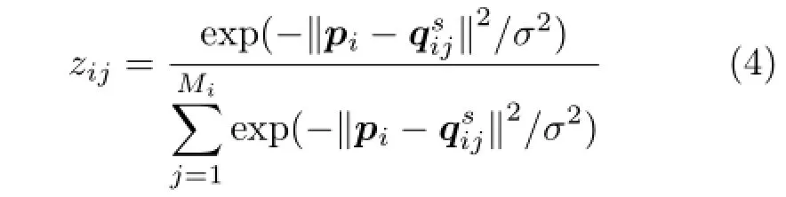
where Miis the number of NNs in Ysof each small patch piin Y，and σ is the standard deviation of noise added on pi.s is the scale factor（see Fig.1）.Note that we apply the same symbol to express column vector corresponding to the patch here.Setting the gradient of the objective function in Eq.（3）to zero can get the update formula of k:

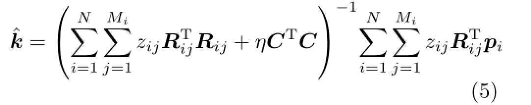
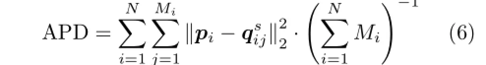
Equation（5）is very similar to the result of Ref.［25］，which can be interpreted as maximum a posteriori（MAP）estimation on k.However，there are at least three essential differentials with respect to Ref.［25］.Firstly，the motivation is different so that Ref.［25］tends to maximize the cross-scale similarity according to NLSS［12］while we minimize the dissimilarity directly according to Ref.［18］.This may not be easy to understand. However，the former leads Michaeli and Irani［25］to form their kernel update formula from physical analysis and interpretation of“optimal kernel”.The latter leads us to obtain kernel update formula from quantitating cross-scale patch dissimilarity and directly minimizing it according to ridge regression ［16］.Secondly，selective patch processing measured bytheaveragegradientamplitude|grad|was adopted to improve the result of blind BKE.Finally，the number of NNs of each small patch piis not fixed which provides more flexibility during solving least square problem.Accordingly，the terminal criterion cannot be the totality of NNs.We use the average patch dissimilarity（APD）as terminal condition of iteration:

It is worth to note that selective patch processing is used to eliminate the effect on BKE caused by smooth patches；we selectively employ structured patches to calculate blur kernel.Specifically，if the average gradient magnitude|grad|of each query patch is smaller than a threshold，then we abandon it.Otherwise，we use it to estimate blur kernel according to Eq.（5）.We typically perform search in the entire image according to Ref.［18］but this could not consume too much time because of a lot of smooth patches being filtered out.

3.2Feature extraction strategy

There is a data preparation stage before dictionary learning when using sparse representation to do SRtask，it is necessary to extract training features from the given input data because different feature extraction strategies will cause very different SR results.The mainstream feature extraction strategies include raw data of an image patch，the gradient of an image patch in x and y directions，and meanremoved patch etc.We adopt the back-projection residuals（BPR）model presented in Ref.［28］for feature extraction（see Fig.3）.

Firstly，we convolve Y with estimated kernel k，and dowm-sample it with s.From the view of minimizing the cross-scale patch dissimilarity，the estimated blur kernel gives us a more accurate downsampling version of Y.In order to make the feature extraction more accurate，we consider the enhanced interpolation of Y′，which forms the source of LR feature space FL.The enhanced interpolation is the result of an iterative back-projection（IBP）operation ［29，30］:

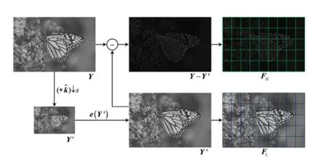
Fig.3　Feature extraction strategy.e（·）represents the enhanced interpolation operation.The down-sampled version Ysis obtained by convolving with estimated kernelˆk and down-sampling with s. LR feature set consists of normalized gradient feature patch extracted from Y′，HR feature set is made up with the raw patches extracted from BPR image Y-Y′.

3.3SR recovery via ASM

Yang et al.［13］accelerated the SR process from two directions:reducing the number of patches and finding a fast solver for L1norm minimization problem.We adopt a similar manner for the first optimization direction，i.e.，a selective patch process （SPP）strategy.However，in order to be consistent with BKE，the criterion of selecting patches is the gradient magnitude|grad|instead of the variance. The second direction Yang et al.headed to is learning a feed-forward neural network model to find an approximated solution for L1norm sparse encoding.We employ ASM to accelerate the algorithm similar with Ref.［17］.It requires us to reformulate the L1norm minimization problem as a least square regression regularized by L2norm of sparse representation coefficients，and adopt the ridge regression（RR）to relieve the computationally demanding problem of L1norm optimization.The problem then comes to be

wheretheparameterµallowsalleviatingthe ill-posed problem and stabilizes the solution.y corresponds to a testing patch extracted from enhanced interpolation version of input image.DLis the LR dictionary trained by ILS-DLA.The algebraic solution of Eq.（8）is given by setting the gradient of objective function to zero，which gives:

where Iis a identity matrix.Then，the same coefficients are used on the HR feature space to compute the latent HR patches，i.e.，x=DHw. Combined with Eq.（9）:

where mapping matrix PMcan be computed offline and DHis computed by Eq.（2）.Equation（10）means HR feature patch can be obtained by LRpatch multiplying with a projection matrix directly，which reduces the time consumption tremendously in practice.Moreover，the feature patches needed to be mapped to HR features via PMwill be further reduced due to SPP.Though the optimization problem constrained by L2norm usually leads to a more relaxative solution，it still yields very accurate SR results because of cross-scale BKE.

4　Experimental results

All the following experiments are performed on the same platform，i.e.，a Philips 64 bit PC with 8.0 GB memory and running a single core of Intel Xeon 2.53 GHz CPU.The core differences between the proposed method and Ref.［16］are the feature extraction and SR recovery.The former is mainly aiming at reducing local projection error and improving the quality of the training samples further.The latter is primarily used to accelerate the reconstruction of the latent HR image.

4.1Experiment settings

We quintessentially perform×2 and×3 SR in our experiments on blind BKE.The parameter settings in BKE stage are partially the same with Refs.［16］and［25］，i.e.，when scale factor s=2，the size of small query patches piand candidate patchesof NNs are typically set to 5×5，while the sizes of“parent”patches qijare set to 9×9 and 11×11；when performing×3 SR，query patches and candidate patches do not change size but“parent”patches are set to be 13×13 patches.Noise standard deviation σ is assumed to be 5.Parameter η in Eq.（3）is set to be 0.25，and matrix C is chosen to be the derivative matrix corresponding to x and y direction of“parent”patches.The threshold of gradient magnitude|grad|for selecting query patches varies in 10-30 according to the different images.In the processing of feature extraction，the enhanced interpolation starts with the bicubic interpolation anddown-samplingoperationisperformedby convolving with estimated blur kernel k，and the back-projection filter k′is set to be a Gaussian kernel with the same size of k.The tradeoff parameterµin Eq.（8）is set to be 0.01 and the number of iteration for dictionary training is 20.

4.2Analysis of the metric in blind BKE

Comparisons for blind BKE usually include the accuracy of the estimated kernels and the efficiency，and these two elaborations have been presented in our previous work［16］in detail.We intend to analyze the impact on blind BKE through discriminating the query patches instead of simply comparing the final results with some related works.The repeated conclusions will be ignored here.We collected patches from three natural image sets（Set2，Set5，and Set14）and found that the values of|grad|and variance mostly fall into the range of［0，100］.So the entire statistical range is set to be［0，100］and the statistical interval for|grad|and variance is typically set to be 10.

We sampled the 500×400“baboon”image and got 236，096 query patches，and 235，928 patches from 540×300“high-street”（dense sampling）.It is distinctly observed that the statistical characteristics of|grad|and variance are very similar with each other in Fig.4.The query patches with threshold ≤30 account for the most proportion for both|grad| and variance，and we could get similar conclusion from other images.However，the relative relation between them reverses around 30（value may be different from images but the reverse determinately exists）.This is an intuitive presentation that why we adopt the|grad|instead of variance as the metric of selecting patches based on the philosophy of dropping the useless smooth patches as many as possible and keeping the structured patches as far as possible.More systemically theoretical explanations could be found in Ref.［18］.

Moreover，the performance of blind BKE is obviously affected by the threshold on|grad|.The optimal kernel was pinned beside the threshold in Fig.4.We can see that the estimated kernel by our method is not close to the ground-truth one infinitely as the threshold increasing because the useful structured patches reduce as well.Usually，the estimated kernel at the threshold of“turning point”is closest to the ground-truth.When the threshold is set to be 0，it actually degenerates to the algorithm of Ref.［25］，which does not give the best result in most instances.In general case，the quality of recovery declines with the increase of|grad|like the second illustration in Fig.4.But there indeed exist special cases like the first illustration in Fig.4 for the PSNRsof recovered images rise firstly and then fell with the threshold increasing.

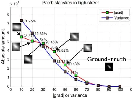
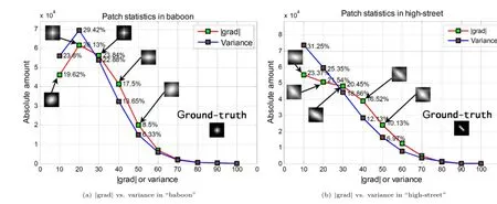
Fig.4　Comparisons between statistical characteristics and threshold effect on estimated kernels.The testing images are“baboon”from Set14 and“high-street”from Set2，and the blur kernels are a Gaussian with hsize=5 and sigma=1.0（9×9）and a motion kernel with length=5，theta=135（11×11）respectively.We only display estimated kernels when threshold on|grad|≤50.

4.3Comparisons for SR recovery

Compared with several currently proposed methods （such as A+ANR［27］and SRCNN［31］etc.），the reconstruction efficiency of our method sometimes is slightly low but almost in the same magnitude. Due to the anchored space mapping，the proposed method was accelerated substantially with regard to some typical sparse representation algorithms like Refs.［11］and［32］.Table 1 and Table 2 present the quantitative comparisons using PSNRs andSRrecoverytimetocompareobjective index and SR efficiency.Four recent proposed methods including Ref.［32］，A+ANR（adjusted anchored neighborhood regression）［27］，SRCNN （super-resolutionconvolutionalneuralnetwork）［31］，and JOR （jointly optimized regressors）［33］arepickedoutastherepresentativeofnonblind methods（presented in Table 1），and three blind methods，NBS（nonparametric blind superresolution）［25］，SAR-NBS（simple，accurate，and robust nonparametric blind super-resolution）［34］，and Ref.［16］are concurrently listed in Table 2 with the proposed method.It's worth noting that PSNR needs reference images as base line.Because the input images are blurred by different blurring kernels so that the observation data is seriously degenerated and non-blind methods usually give very bad results in this case，we referred the recovered images to the blurred input images.The average PSNRs and running time are collected（×2 and×3）over four image sets（Set2，Set5，Set14，and B100）. Besides，we set the threshold on|grad|around to the“turning point”adaptively for the best BKE estimation instead of pinning it to a fixed number （e.g.，10 in Ref.［16］）.The methods listed in Table 1 and Table 2 are identical to the methods presented in Figs.5-8.

As shown in Table 1 and Table 2，the proposed algorithm obtained higher objective evaluation than other blind or non-blind algorithms in both s=2 and/or s=3 case.For fairness，it excludes the time of preparing data and training dictionaries for all of these methods.Firstly，four non-blind methods in Table 1 fail to recover real images when the inputs are degraded seriously though some of them provided very high speed.And，both the accuracy and efficiency of estimating kernels via Michaeli et al.［25］are not high enough which has been illustrated in Ref.［16］，and SR recovery performed by Ref.［11］is very time-consuming. While the same process of BKE with us was executed in Ref.［16］（fixed threshold on|grad|），the SR reconstruction with SPP is essentially still lowefficiency.The proposed method adopted adaptive |grad|threshold to improve the quality of BKE and the enhanced interpolation on input images reduced the mapping errors brought by estimated kernels further.On the other hand，ASM increased the speed of the algorithm in essence.This is mainlydue to the adjustment of the objective function and the constraint conversion from L0/L1norm to L2norm.Actually，the improvement of our method is not only reflected in SR recovery stage，but also reflected in BKE （through SPP）and dictionary training（through ILS-DLA）which are not usually mainly concerned by most of researchers.But these preprocessing procedures are still very different when big data need to be processed.

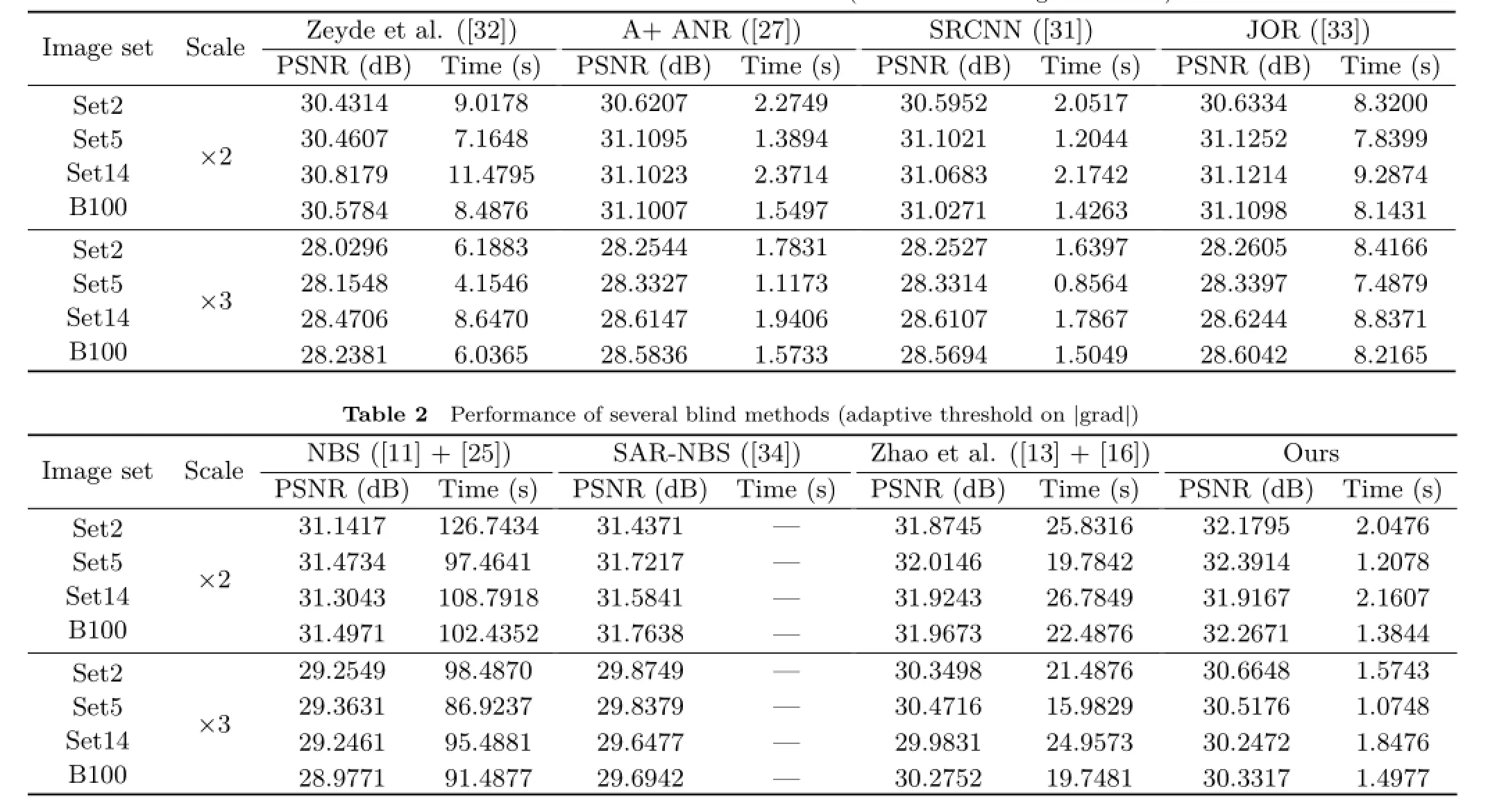
Table 1　Performance of several non-blind methods（without estimating blur kernel）

Figures 5-8 show the visual comparisons between several typical SR algorithms and our method.For layout purpose，all images are diminished when inserted in the paper.Still note that the input images of all algorithms are obtained through reference images blurred with different blur kernel. Namely，input image data is set to be of low quality in our experiments for the sake of simulating many actual application scenarios.Though it is well known that non-blind SR algorithms presented intheillustrationsareefficientformanySR tasks，they fail to offset the blurring effect in testing images without a more precise blurring kernel.There is also significant difference about the estimated kernels and reconstruction results among blind algorithms.The BKE process of Ref.［25］is actually close to our method when the threshold on|grad|is 0 and the criterion for iteration is MSE.Shao et al.［34］solved the blur kernel and HR image simultaneously by minimizing a bi-L0-L2-norm regularized optimization problem with respect to both an intermediate super-resolved image and a blur kernel，which is extraordinarily time-demanding （so not shown in Table 1）.More important is that the fitting problem caused by useless smooth patches still exists in these methods.Although the idea of our method is simple，it could avoid the fitting problem by dropping the smooth query patches reasonably according to the internal statistics of a single natural image.

Figures 9 and 10 present SR recovery results of other two real images（“fence”and“building”），which were captured by our cell-phone with slightly joggle and motion.It is easily noticed that all blind methods produce a better result than nonblind methods which even can not offset the motion deviation basically.Comparing Fig.9（f）-Fig.9（i）and Fig.10（f）-Fig.10（i），we can find the visible difference in estimated kernels and recovered results produced by different blind methods.Particularly，SAR-NBS tends to overly sharpen the high frequency region and gives obvious distortion in final images. The results of Zhao et al.［16］look more realistic but the reconstruction accuracy is not high enough compared with our approach.

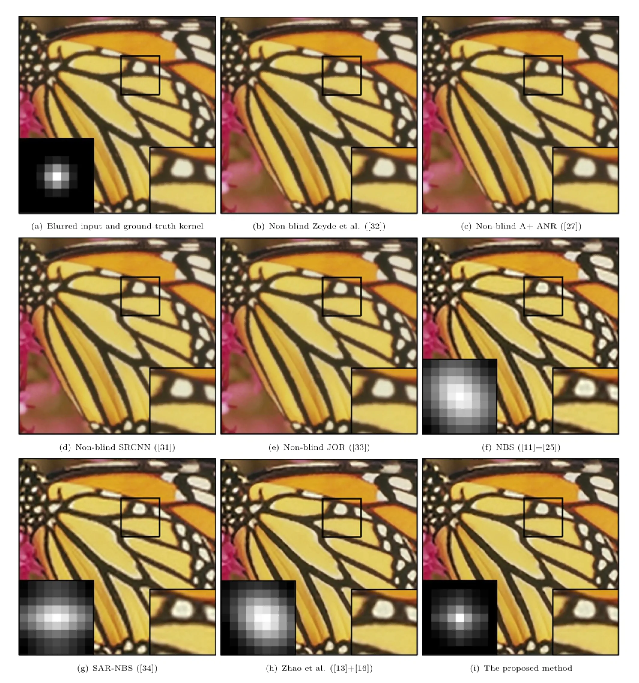
Fig.5　Visual comparisons of SR recovery with low-quality“butterfly”image from Set5（×2）.The ground-truth kernel is a 9×9 Gaussian kernel with hsize=5 and sigma=1.25，and threshold on|grad|is 18.

5　Conclusions

We proposed a novel single image SR processing framework aiming at improving the SR effect and reducing SR time consumption in this paper.The proposed algorithm mainly consists of blind blur kernel estimation and SR recovery.The former is based on the idea of minimizing dissimilarity of cross-scale image patches，which leads us to obtain kernel update formula by quantitating crossscale patch dissimilarity and directly minimizing it according to least square method.The reduction of SR time mainly relies on an ASM processwithLR/HRdictionariestrainedbyILS-DLA algorithms a selective patch processing strategy measured by|grad|.Therefore，the SR effect is mainly guaranteed by improving the quality of training samples and the efficiency of SR recovery is mainly guaranteed by anchored space mapping and selective patch processing.They ensure the improvement of time performance via reducing the number of query patches and translating L1norm constrained optimization problem into L2norm constrained anchor mapping process.Under the equal conditions，all above-mentioned processes makeourSRalgorithmachievebetterresults than several outstanding blind and non-blind SR approaches proposed previously with a much higher speed.

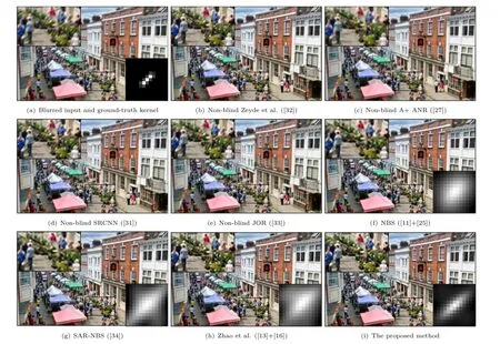
Fig.6　Visual comparisons of SR recovery with low-quality“high-street”image from Set2（×3）.The ground-truth kernel is a 13×13 motion kernel with len=5 and theta=45，and threshold on|grad|is 24.

Acknowledgements

We would like to thank the authors of Ref.［34］，Mr.Michael Elad and Mr.Wen-Ze Shao，for their kind help in running their blind SR method［34］，which thus enables an effective comparison with their method.This work is partially supported by National Natural Science Foundation of China （GrantNo.61303127），WesternLightTalent Culture Project of Chinese Academy of Sciences （Grant No.13ZS0106），Project of Science and Technology Department of Sichuan Province（Grant Nos.2014SZ0223 and 2015GZ0212），Key Program ofEducationDepartmentofSichuanProvince （Grant Nos.11ZA130 and 13ZA0169），and the innovation funds of Southwest University of Science and Technology（Grant No.15ycx053）.

References

［1］Freedman，G.；Fattal，R.Image and video upscaling fromlocalself-examples.ACMTransactionson Graphics Vol.30，No.2，Article No.12，2011.

［2］Babacan，S.D.； Molina，R.； Katsaggelos，A. K.Parameter estimation in TV image restorationusing variational distribution approximation.IEEE Transactions on Image Processing Vol.17，No.3，326-339，2008.

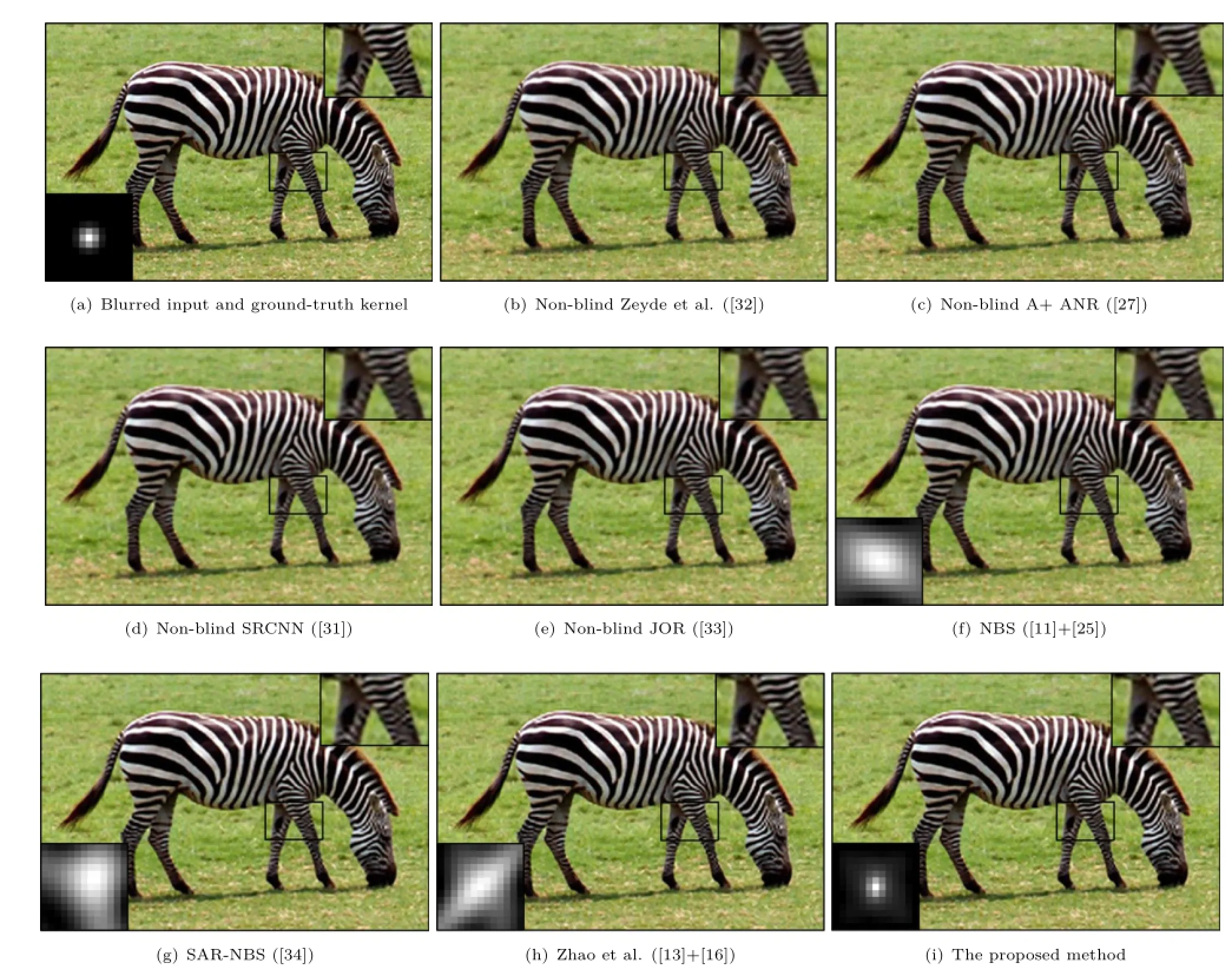
Fig.7　Visual comparisons of SR recovery with low-quality“zebra”image from Set14（×3）.The ground-truth kernel is a 13×13 Gaussian kernel with hsize=5 and theta=1.25，and threshold on|grad|is 16.

［3］Babacan，S.D.；Molina，R.；Katsaggelos，A.K. Total variation super resolution using a variational approach.In:Proceedingsofthe15thIEEE International Conference on Image Processing，641-644，2008.

［4］Babacan，S.D.； Molina，R.；Katsaggelos，A. K.VariationalBayesiansuperresolution.IEEE Transactions on Image Processing Vol.20，No.4，984-999，2011.

［5］Sun，J.；Xu，Z.；Shum，H.-Y.Image super-resolution using gradient profile prior.In:Proceedings of IEEE Conference on Computer Vision Pattern Recognition，1-8，2008.

［6］Freeman，W.T.；Jones，T.R.；Pasztor，E.C.Examplebased super-resolution.IEEE Computer Graphics and Applications Vol.22，No.2，56-65，2002.

［7］Sun，J.；Zheng，N.-N.；Tao，H.；Shum，H.-Y. Image hallucination with primal sketch priors.In: Proceedings of IEEE Computer Society Conference on Computer Vision and Pattern Recognition，Vol.2，729-736，2003.

［8］Chang，H.；Yeung，D.Y.；Xiong，Y.Super-resolution through neighbor embedding.In:Proceedings of IEEE Computer Society Conference on Computer Vision and Pattern Recognition，275-282，2004.

［9］Roweis，S.T.；Saul，L.K.Nonlinear dimensionality reduction by locally linear embedding.Science Vol. 290，No.5，2323-2326，2000.

［10］Bevilacqua，M.；Roumy，A.；Guillemot，C.；Morel，M.-L.A.Low-complexity single-image super-resolution basedonnonnegativeneighborembedding.In: Proceedingsofthe23rdBritishMachineVision Conference，135.1-135.10，2012.

［11］Yang，J.；Wright，J.；Huang，T.；Ma，Y.Image super-resolution as sparse representation of raw image patches.In:Proceedings of IEEE Conference on Computer Vision and Pattern Recognition，1-8，2008. ［12］Glasner，D.；Bagon，S.；Irani，M.Super-resolution from a single image.In:Proceedings of IEEE 12thInternational Conference on Computer Vision，349-356，2009.

［13］Yang，J.；Wang，Z.；Lin，Z.；Cohen，S.；Huang，T.Coupled dictionary training for image superresolution.IEEE Transactions on Image Processing Vol.21，No.8，3467-3478，2012.

［14］Yang，J.；Wright，J.；Huang，T.；Ma，Y.Image super-resolutionviasparserepresentation.IEEE Transactions on Image Processing Vol.19，No.11，2861-2873，2010.

［15］He，L.；Qi，H.；Zaretzki，R.Beta process joint dictionary learning for coupled feature spaces with applicationtosingleimagesuper-resolution.In: Proceedings of IEEE Conference on Computer Vision and Pattern Recognition，345-352，2013.

［16］Zhao，X.；Wu，Y.；Tian，J.；Zhang，H.Single image super-resolution via blind blurring estimation and dictionary learning.In:Communications in Computer and Information Science，Vol.546.Zha，H.；Chen，X.；Wang，L.；Miao，Q.Eds.Springer Berlin Heidelberg，22-33，2015.

［17］Timofte，R.；De，V.；VanGool，L.Anchored neighborhood regression for fast example-based superresolution.In:Proceedings of IEEE International Conference on Computer Vision，1920-1927，2013.

［18］Zontak，M.；Irani，M.Internal statistics of a single natural image.In:Proceedings of IEEE Conference on Computer Vision and Pattern Recognition，977-984，2011.

［19］Yang，C.-Y.；Huang，J.-B.；Yang，M.-H.Exploiting self-similarities for single frame super-resolution.In: LectureNotesinComputerScience，Vol.6594. Kimmel，R.；Klette，R.；Sugimoto，A.Eds.Springer Berlin Heidelberg，497-510，2010.

［20］Zoran，D.；Weiss，Y.Fromlearningmodelsof natural image patches to whole image restoration. In:Proceedings of IEEE International Conference on Computer Vision，479-486，2011.

［21］Hu，J.；Luo，Y.Single-image superresolution based on local regression and nonlocal self-similarity.Journal of Electronic Imaging Vol.23，No.3，033014，2014.

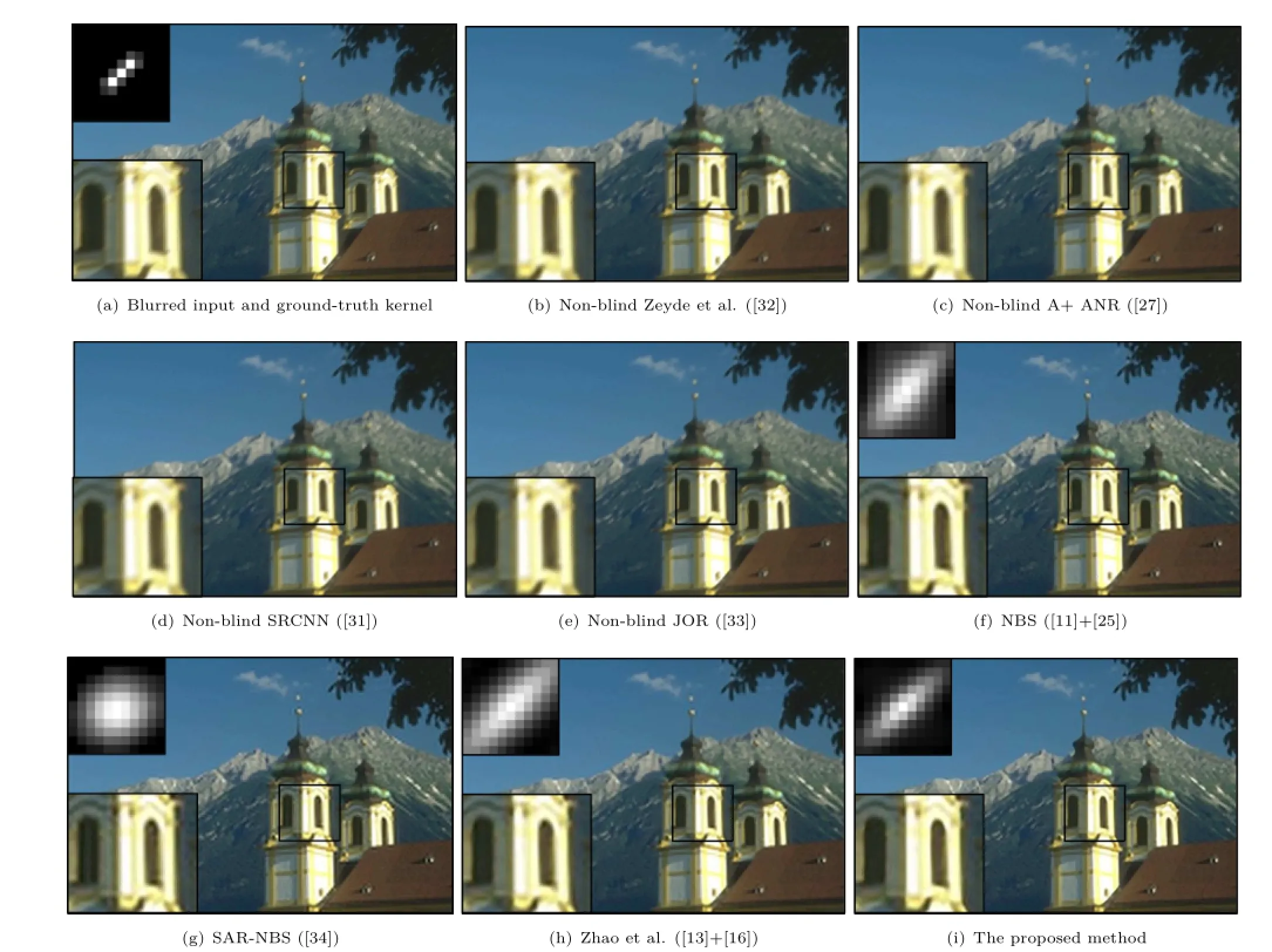
Fig.8　Visual comparisons of SR recovery with low-quality“tower”image from B100（×2）.The ground-truth kernel is a 11×11 motion kernel with len=5 and tehta=45，and threshold on|grad|is 17.

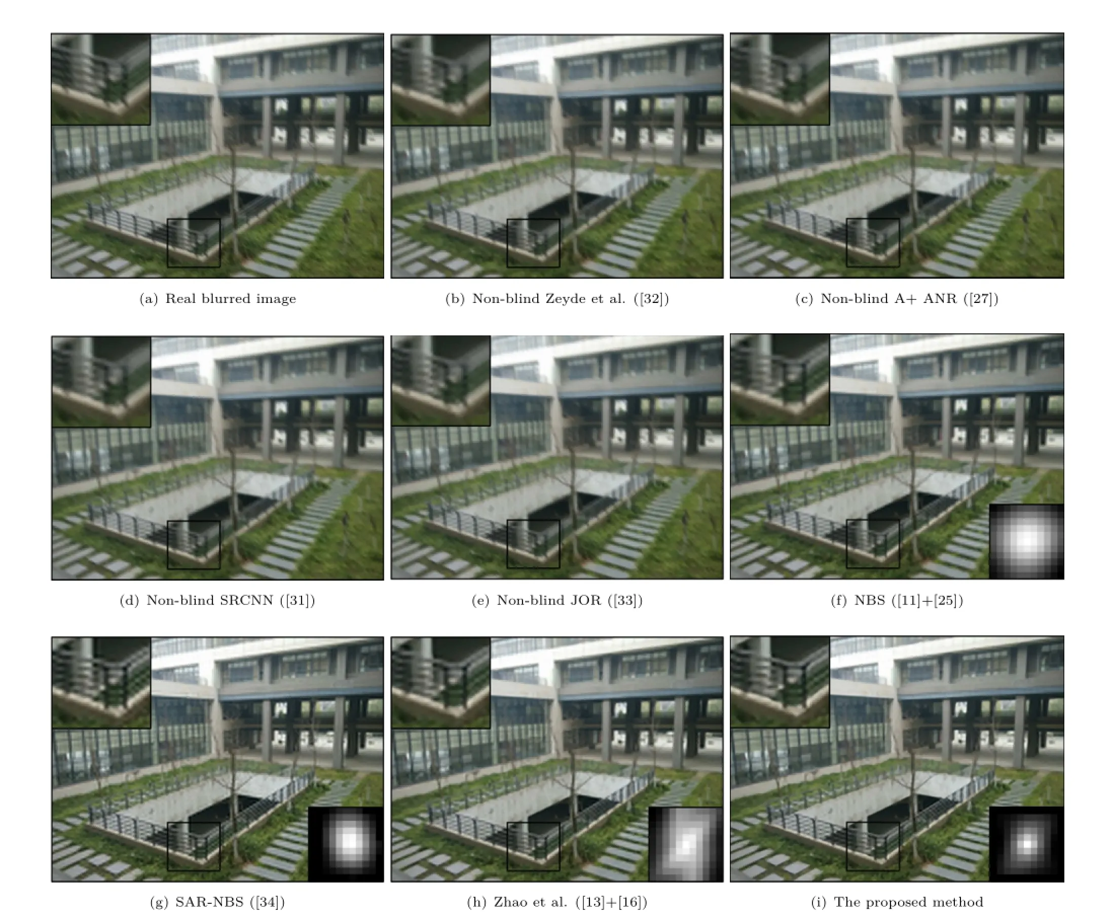
Fig.9　Visual comparisons of SR recovery with real low-quality image“fence”captured with slight joggle（×2）.Threshold on|grad|is 21.

［22］Zhang，Y.；Liu，J.；Yang，S.；Guo，Z.Joint imagedenoisingusingself-similaritybasedlowrankapproximations.In:ProceedingsofVisual Communications and Image Processing，1-6，2013.

［23］Michaeli，T.；Irani，M.Blind deblurring using internal patch recurrence.In:Lecture Notes in Computer Science，Vol.8691.Fleet，D.；Pajdla，T.；Schiele，B.；Tuytelaars，T.Eds.Springer International Publishing，783-798，2014.

［24］Guillemot，C.；LeMeur，O.Imageinpainting: Overview and recent advances.IEEE Signal Processing Magazine Vol.31，No.1，127-144，2014.

［25］Michaeli，T.；Irani，M.Nonparametric blind superresolution.In:Proceedings of IEEE International Conference on Computer Vision，945-952，2013.

［26］Engan，K.；Skretting，K.；Husøy，J.H.Family of iterative LS-based dictionary learning algorithms，ILSDLA，for sparse signal representation.Digital Signal Processing Vol.17，No.1，32-49，2007.

［27］Timofte，R.；De Smet，V.；Van Gool，L.A+:Adjusted anchored neighborhood regression for fast superresolution.In:Lecture Notes in Computer Science，Vol.9006.Cremers，D.；Reid，I.；Saito，H.；Yang，M.-H.Eds.Springer International Publishing，111-126，2014.

［28］Bevilacqua，M.；Roumy，A.；Guillemot，C.；Morel，M.-L.A.Super-resolution using neighbor embedding of back-projection residuals.In:Proceedings of the 18th International Conference on Digital Signal Processing，1-8，2013.

［29］Irani，M.；Peleg，S.Motionanalysisfor imageenhancement:Resolution， occlusion， and transparency.Journal of Visual Communication and Image Representation Vol.4，No.4，324-335，1993.

［30］Irani，M.；Peleg，S.Improving resolution by image registration.CVGIP:Graphical Models and Image Processing Vol.53，No.3，231-239，1991.

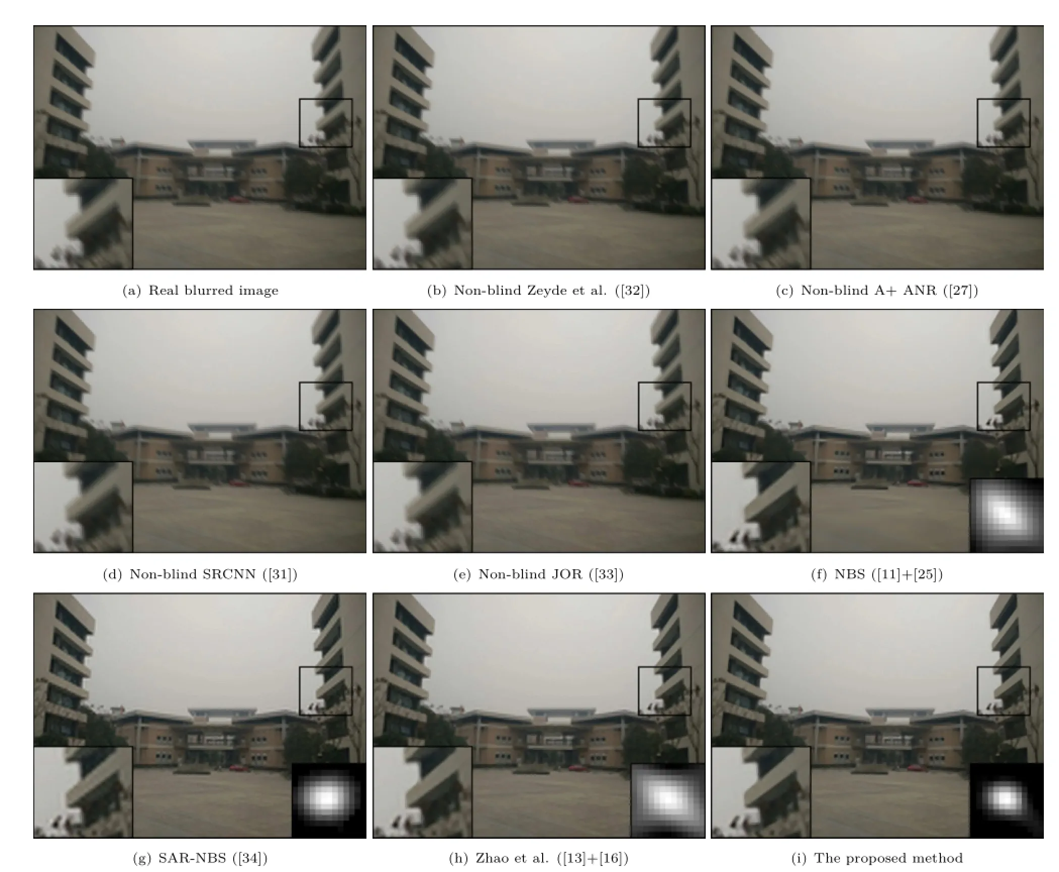
Fig.10　Visual comparisons of SR recovery with real low-quality image“building”captured with slight motion（×2）.Threshold on|grad|is 26.

［31］Dong，C.； Chen，C.L.； He，K.； Tang，X. Learning a deep convolutional network for image super-resolution.In:Lecture Notes in Computer Science，Vol.8692.Fleet，D.；Pajdla，T.；Schiele，B.；Tuytelaars，T.Eds.Springer International Publishing，184-199，2014.

［32］Zeyde，R.；Elad，M.；Protter，M.On single image scaleup using sparse-representations.In:Lecture Notes in Computer Science，Vol.6920.Boissonnat，J.-D.；Chenin，P.；Cohen，A.et al.Eds.Springer Berlin Heidelberg，711-730，2010.

［33］Dai，D.；Timofte，R.；Van Gool，L.Jointly optimized regressorsforimagesuper-resolution.Computer Graphics Forum Vol.34，No.2，95-104，2015.

［34］Shao，W.-Z.；Elad，M.Simple，accurate，and robust nonparametric blind super-resolution.In:Lecture NotesinComputerScience，Vol.9219.Zhang，Y.-J.Ed.Springer International Publishing，333-348，2015.

Xiaole Zhao received his B.S.degree in computer science from the School of Computer Science and Technology，Southwest University of Science and Technology（SWUST），China，in 2013. HeisnowstudyingintheSchool of Computer Science and Technology，SWUST for his master degree.His main research interests include digital image processing，machine learning，and data mining.

Yadong Wu now is a full professor with the School of Computer Science and Technology，Southwest University of Science and Technology（SWUST），China.He received his B.S.degree in computer science from Zhengzhou University，China，in 2000，and M.S. degree in control theory and controlengineering from SWUST in 2003.He got his Ph.D.degree in computer application from University of Electronic Science and Technology of China.His research interest includes image processing and visualization.

Jinsha Tian received her B.S.degree inHebeiUniversityofScienceand Technology，China，in 2013.She is now studying in the School of Computer ScienceandTechnology， Southwest University of Science and Technology （SWUST），China for her master degree. Hermainresearchinterestsinclude digital image processing and machine learning.

HongyingZhangnowisafull professor with the School of Information Engineering，Southwest University of ScienceandTechnology（SWUST），China.She received her B.S.degree in applied mathematics from Northeast University，China，in 2000，and M.S. degree in control theory and control engineering from SWUST in 2003.She got her Ph.D. degree in signal and information processing from University of Electronic Science and Technology of China，in 2006.Her research interest includes image processing and biometric recognition.

Open AccessThe articles published in this journal aredistributedunderthetermsoftheCreative CommonsAttribution4.0InternationalLicense （http://creativecommons.org/licenses/by/4.0/），which permits unrestricted use，distribution，and reproduction in any medium，provided you give appropriate credit to the original author（s）and the source，provide a link to the Creative Commons license，and indicate if changes were made.

Other papers from this open access journal are available free of charge from http://www.springer.com/journal/41095. To submit a manuscript，please go to https://www. editorialmanager.com/cvmj.

Research Article

Single image super-resolution via blind blurring estimation and anchored space mapping