Critical Behaviors and Finite-Size Scaling of Principal Fluctuation Modes in Complex Systems∗

Xiao-Teng Li(李晓腾)and Xiao-Song Chen(陈晓松)

Institute of Theoretical Physics,Key Laboratory of Theoretical Physics,Chinese Academy of Sciences,P.O.Box 2735,Beijing 100190,China

School of Physical Sciences,University of Chinese Academy of Sciences,No.19A Yuquan Road,Beijing 100049,China

1 Introduction

Complex system refers to systems with enormous agents interacting with each other.From microscopic interactions under different external conditions,emergent phenomena and collective behaviors appear in a macroscopic scale.The interactions in complex systems have often multiple scales of length and time and are of character of complexity.

In recent decades,datasets of a variety of complex systems become available.Data analysis and techniques for data analysis have aroused broad interests of scientists.[1−2]Among all data analysis techniques,principal component analysis is the most fundamental one with various applications,such as dimension reducing,[3−4]clustering[5]and eigen-mode extraction.[6−12]From data of a complex system consisting ofNagents,the correlation between any two agents and therefore anN×Ncorrelation matrix can be obtained.Using the pricipal component analysis,we can getNindependent principal fluctuation modes of agents from theN×Ncorrelation matrix.The fluctuations of whole system are dominated usually by a few of principla fluctuation modes.[6]From the characters of these principal fluctuation modes,we can have a good understanding of global properties.

For thermodynamic systems with finite size,their thermodynamic functions satisfy the finite-size scaling form in the neighborhood of a critical point.[13−14]This can be used to identify the continuous phase transition in a finite system.If thermodynamic functions of a finite system follow finite-size scaling laws,there is a continuous phase transition in the system.With the critical exponents determined from finite-size scaling forms,the universality class of the continuous phase transition can be con fi rmed.

For many complex systems,their principal fluctuation modes instead of thermodynamic functions can be investigated usually.The studies of the critical behaviors of principal fluctuation modes are of great interest.We like to know the finite-size behaviors of principal fluctuation modes near a critical point.In this article,we propose a finite-size scaling form of principal fluctuation modes.We can use this scaling form to study the critical phenomena of complex systems.

Using the Is ing model on a two-dimensional simple square lattice[15]as an example,we will investigate the critical behaviors of principal fluctuation modes.It is found that the principal fluctuation modes near critical point show critical behaviors and satisfy the finite-size scaling we proposed.From eigen values of principal fluctuation modes,we can calculate the second moment correlation length which follows a finite-size scaling form.

Our paper is organized as follows.In Sec.2,we introduce the principla fluctuation modes of complex systems and propose a finite-size scaling form for them.Taking the Is ing model on a two-dimensional square lattice as an example,we investigate principal fluctuation modes and their finite-size scaling behaviors near the critical point in Sec.3.The second moment correlation length is calculated from the eigen values of principal fluctuation modes in Sec.4.Finally,we make conclusions in Sec.5.

2 Finite-Size Scaling of Principal Fluctuation Modes in Complex Systems

2.1 Principla Fluctuation Modes of Complex Systems

In a complex system consisting ofNagents,agents interact with each other and they are correlated.define a snapshot “I” of the system as con figuration “I”,the state of an agentiis characterized bySi(I).From all con figurations of the system,the average state of agentiis calculated as

whereRis the number of the con figurations.The agentihas a fluctuationδSi(I)≡Si(I)−⟨Si＞in the con figuration“I”.The correlation between agentsiandjis defined as

Withcijas its elements,anN×Ncorrelation matrixCis introduced.There areNeigenvectors and eigenvalues for the correlation matrixC.The eigenvector corresponding an eigenvalueλnis written as

which satisfies the equation

All eigenvectors are normalized and orthogonal to each other.Any eigenvectorsbnandblfollow the condition

whereδnl=0 whenn=landδnl=1 ifn=l.

From an eigenvectorbn,we can define a principal fluctuation mode

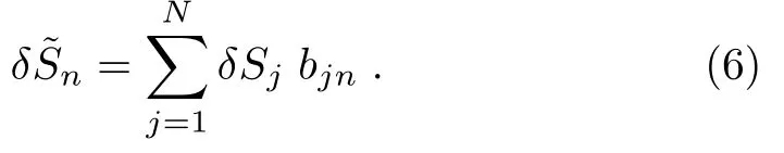
For a transform matrixBdefined by elementsBin=bin,there are the relationsB·BT=IandBT=B−1.Equation(4)can be rewritten asC·B=B·Λ,where Λ is a diagonal matrix with elements Λnl=λnδnl.

Using the orthogonal condition of Eq.(5),we get the correlation between principal fluctuation modes

There is no correlation between different principal fluctuation modes and the mean square of a principal fluctuation modeis equal toλn.

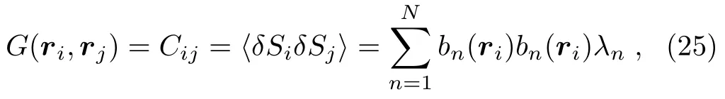
From theNeigenvalues of correlation matrixCand their eigenvectors,we can calculate the correlation between agentiandjas

whereQij|n=binbjnis the link strength between agentiandjofn-th principla fluctuation mode.We can expect that the correlation length of a complex system is related to the eigenvalues of its principal fluctuation modes.

We define the state of system as

The total correlation of an agentican be calculated as

whereis the total link of the agentiinn-th principla fluctuation mode.The average ofDigives the susceptibility

where=ijQij|n/N.is the average link ofn-th principal fluctuation mode.We can consider the eigen valueλnas the susceptibilty ofn-th principal fluctuation mode.The susceptibility of system is the sum of all eigen valueλnwith a weight factor¯Qn.

Corresponding toNinteracting agents in the system,there areNindependent principla fluctuation modes.In some cases,the susceptibility is dominated just by a few of principla fluctuation modes.From the investigations of several principla fluctuation modes,we can catch the global behaviors of system.

2.2 Finite-Size Scaling of Principal Fluctuation Modes

According to the finite-size scaling theory of critical phenomena,[13−14]the susceptibility of a finie system with sizeLhas the following finite size scaling form

wheret=(T−Tc)/Tcis the reduced temperature andTcis the critical temperature.

Because of the relation between susceptibility and eigen valuesλnof principal fluctuation modes in Eq.(10),we suppose thatλnfollow a finite-size scaling form as

for a few of dominant principal fluctuation modes.We anticipate that the exponentζnis equal to the ratio of critical exponentγ/νand is independent ofn.

The finite-size scaling form in Eq.(12)can be used to investigate the critical behaviors of complex systems.

3 Finite-Size Scaling of Principal Fluctuation Modes in Two-Dimensional Is ing Model

Here we use the Is ing model on a two-dimensional simple square lattice with zero external field to study its principal fluctuation modes.For the two-dimensional square lattice,periodic boundary conditions are taken.There areNspins,which interact each other and have the Hamiltonian

where interactions are restricted to the nearest neighbors.The spinSiat siteican point up or down and hasSi=±1 respectively.A con figuration with{Si}=(S1,S2,...,SN)appears with a probability

whereβ=1/(kBT)andkBis the Boltzmann’s constant.The statistical average of any observableA({Si})is calculated as

where the summation can be done for the sampled con figurations{Si}simulated by the Wol ffalgorithm.

In a finite Is ing model,there is no symmetry breaking.We have always=0 if all con figurations are considered in the average.Correspondingly,the average of total magnetization

To characterize the appearance of ferromagnetic phase,we restrict the statistical average to the con figurations with positive total magnetization.In this case,the averages=＞andm=are nonzero.In the bulk limitN→∞,m=0 for temperatureT>Tcandm>0 for temperatureT0 indicate the appearance of ferromagnetic phase.

If the total magnetizationMis negative after a Monte Carlo step,we make a fl ipSi→−Sito all spins so thatMbecome positive again.For this fl ip,the total energy of the Is ing model is unchanged.

Using only the con figurations with positive total magnetization,we can define anN×Ncorrelation matrixCwith elements

For the correlation matrixC,there areNeigenvaluesλiandNcorresponding eigenvectorsbi.,wherei=1,2,...,N.An eigen vectorbiis the field defined on a two-dimensional simple square lattice.The principal fluctuation modeis the summation of all fluctuationsδSjat the sitejwith coefficentbjn.

3.1 Finite-Size Scaling at the Critical Point

At the critical pointT=Tcof two-dimensional Is ing model,the finite-size scaling form of principal fluctuation modes becomes

The logarithm of this equation gives

so that the log-log plot ofλversusLatT=Tcis a straight line with slope equat to the exponentζ.

We find that the eigen valuesλnhave degeneracy.These results are shown in Fig.1.In the first degerate group,eigen valuesλ2,λ3,λ4,andλ5are equal.The eigen valuesλ6,λ7,λ8andλ9in the second degerate group have the same results within the range of error.The degeneracy here is the consequence of the symmetry in simple square lattice,which will be discussed in Subsec.3.4.

From the slopes of straight lines in Fig.1,we can get the exponentζn.The results are summarized in Table 1.As we suspected in the last section,the exponentζnis independent ofnand equal to the the exponent ratioγ/ν=7/4 of two-dimensional Is ing model.

Fig.1 Log-Log plot of λnversus L at T=Tcfor n=1,2,...,9.The critical exponents ζnare given by the slopes of the linear lines.

Table 1 Critical exponent of n-th eigenvalue λn.

3.2 Finite-Size Scaling Functions of Principal Fluctuation Modes

At temperatures around the critical pointTc,the largest eigen valuesλ1(L,t)simulated for system sizesL=16,32,64 are shown in Fig.2(a).According to the finite-size scaling form of Eq.(12),the Monte Carlo data ofλ1(L,t)should collapse into one curve of scaling variabletL1/νafter multiplyingL−ζ1,which is demonstrated in Fig.2(b).

In Fig.3(a),the degenerate eigen valuesλ2(L,t),λ3(L,t),λ4(L,t)andλ5(L,t)are shown with respect to temperaureTfor system sizesL=16,32,64.The finite-size scaling functionsofn=2,3,4,5 are presented in Fig.3(b).

In Fig.4,we present the degenerate eigen valuesλ6(L,t),λ7(L,t),λ8(L,t),andλ9(L,t)on the left and their finite-size scaling functions on the right.

Fig.2 Eigenvalue λ1(L,t)is shown as a function of temperature T for system sizes L=16,32,64 in the left.Using λ1(L,t)L−ζ1= (tL1/ν),different curves in the left collapse into one curve in the right.

Fig.3 (a)Degenerate eigen values λ2(L,t), λ3(L,t),λ4(L,t)and λ5(L,t)versus temperature T for system sizes L=16,32,64. (b) finite-size scaling functions λn(L,t)L−ζn= (tL1/ν)of n=2,3,4,5.

Fig.4 (a)Degenerate eigen values λ6(L,t), λ7(L,t),λ8(L,t)and λ9(L,t)versus temperature T for system sizes L=16,32,64. (b)Finite-size scaling functions λn(L,t)L−ζn= (tL1/ν)of n=6,7,8,9.

3.3 Eigenvalue Ratios of Principal Fluctuation Modes

Since the eigenvaluesλn(L,t)of different principal fluctuation modes follow the finite-size scaling form Eq.(12)with the same exponentζn,the eigenvalue ratioRn/l(L,t)≡λn(L,t)/λl(L,t)has the finite-size scaling form

At critical point witht=0,the ratioRn/l(L,0)=fn/l(0)is independent of system sizeL.This property ofRn/lcan be used to determine the critical point from its fixed point.As analogous to the cumulant ratio of magnetization,we anticipate that the finite-size scaling functionfn/l(tL1/ν)is universal.The eigenvalue ratiofn/l(0)at the critical point is a universal constant.

In Fig.5,the eigenvalue ratiosR1/l(L,t)ofλ1toλlforl=2,3,4,5 are shown with respect to temperatureTand the scaling variabletL1/νin the left and right respectively.We find a perfect finite-size scaling for the Monte Carlo data of different sytem sizesL=16,32,64.

The eigenvalue ratiosR1/l(L,t)ofn=6,7,8,9 are presented in Fig.6.With temperatureTas variable,the curvesR1/lof system sizesL=16,32,64 di ff er.After using the scaling variabletL1/ν,the different curves ofR1/lin the left collapse into one curve in the right.

Fig.5 Eigenvalue ratio λ1/λlof l=2,3,4,5 versus temperature T and the scaling variable tL1/νfor system sizes L=16,32,64.Monte Carlo data of different L demonstrate a fixed point at the critical point.

Fig.6 Eigenvalue ratio λ1/λlfor n=6,7,8,9 versus temperature T and the scaling variable tL1/νfor system sizes L=16,32,64.Monte Carlo data of different system sizes have a fixed point at Tc.

3.4 Space Distribution of Principal Fluctuation Modes

From theN-dimensional eigen vectorbn,we can get the space distributionbn(r)ofn-th principal fluctuation mode.The space distribution functionbn(r)satisfies the normalization conditio

To characterize the space distributionbn(r),we make the following Fourier analysis

The summation over vectorkin Eq.(22)is done fork=(kx,ky)=((2π/L)nx,(2π/L)ny)and−π

Fig.7 Rescaled space distributions of principla fluctuation modes˜bn(r)=L×bn(r)of groups n=1,n=2,3,4,5 and n=6,7,8,9 at the critical point T=Tcfor system size L=128.

In Fig.7,the rescaled space distribution(r)=L×bn(r)is presented in three groups ofn=1,n=2,3,4,5 andn=6,7,8,9.For the first groupn=1,the space distribution is very fl at and all spins of the system fluctuate synchronously.The space distributions of the second group withn=2,3,4,5 have one peak and one valley.In the third group withn=6,7,8,9,the space distribution functions of principal fluctuation modes have two peaks and two valleys.

Before we make the Fourier analyses of the space distribution of principal fluctuation modes,we show the Fourier space of two-dimensional square lattice with periodic boundary conditions in Fig.8.

Fig.8 (Coloronline)Fourierspace((2π/L)nx,(2π/L)ny)of two-dimensional square lattice with periodic boundary conditions.The sites with the same color have equal|k|.

The first principal fluctuation modeb1(r)has only(0,0)componen so that(0)|2=1.0000.

The principal fluctuation modes of the second group consist of four components withk=±(0,(2π/L))andk=±(2π/L,0).We present the Fourier components(±(2π/L,0))|2and(±(0,2π/L))|2ofn=2,3,4,5 in Table 2.Within the error range of Monte Carlo data,the normalization condition in Eq.(24)is satisfied forn=2,3,4,5.

In the third group,principal fluctuation modes consist of four components ofk=±(2π/L,2π/L)andk=±(2π/L,−2π/L).The Fourier components of principal fluctuation modebn(r)are given in Table 2 forn=6,7,8,9 and satisfy the normalization condition of Eq.(24).

Table 2 Fourier components of principal fluctuation modes in the second and the third group at the critical point Tcand system size L=128.

4 The Second Moment Correlation Lenght and Principal Fluctuation Modes

From the correlation matrixCij,we can get the correlation function

which covers the contributions of all principal fluctuation modes.With the correlation function,the second moment correlation length squared can be calculated as

In the bulk limitL→∞,vectorkof the Fourier space is continuous and the second moment correlation can be written as[16]

where the Fourier coefficien of the correlation function

and can be calculated as

For finite system,vectorkof the Fourier space is discrete and the definition of the second moment correlation lenght in Eq.(27)is replaced by

The second moment correlation length in thexdirection is calculated atk=±(2π/L,0)where

Therefore,we get the second moment correlation length of thex-direction

which follows the finite-size scaling form

with

Similarly,the Fourier coefficient

Therefore,the second moment correlation length in they-direction

Our Monte Carlo simulation results ofare shown versus temperatureTand for different system sizes in Fig.9(a).The second moment correlation length scaled is presented with respect to the scaling variabletL1/νin Fig.9(b).The different curves ofL=16,32,64 in the left collapse into one curve in the right.

Fig.9 Second moment correlation length squared ξ210 of the x-direction.(a)ξ210as function of temperature for L=16,32,64.(b)ξ10/L2as function of the scaling variable tL1/ν.

According to Eq.(30),the second moment correlation length of the(1,1)-direction can be calculated as

The Monte Carlo results ofand its scaling functionξ11/L2are given in Fig.10.Similarly,the second moment correlation length of the(1,–1)-direction is equal toξ11.

After making a comparison of Fig.10 with Fig.9,we can conclude that the second moment correlation length of the(1,1)-direction is different from that of the(1,0)-direction.Therefore,the second moment correlation length in the two-dimensional square lattice is anisotropic.This is in agreement with the anisotropy of the exponential correlation length.

Fig.10 Second moment correlation length squared ξ211 of the(1,1)-direction.(a)ξ211as function of temperature for L=16,32,64.(b)ξ11/L2as function of the scaling variable tL1/ν.

5 Conclusions

For the data of a complex system consisting ofNagents,the correlations between all agents can be calculated.With the correlations as elememnts,anN×Ncorrelation matrixCof the complex system can be obtained.TheNeigenvectors ofCdefine theNprincipal fluctuation modes of the complex system.The mean square of a principal fluctuation mode is equal to its corresponding eigenvalue.It is observed often that the fluctuations of complex system are dominated just by a few of principal fluctuation modes with larger eigenvalues.In this case,the complex system can be studied by investigating some of theNprincipal fluctuation modes.From the dominant principal fluctuation modes,the global properties of complex systems,such as susceptibility,can also be calculated.

Near the critical point of a complex system,the mean squares of dominant principal fluctuation modes are anticipated to have critical behaviors similar to that of susceptibility.For a finite complex system near its critical point with small reduced temperaturet=(T−Tc)/Tc,the eigenvalues of the dominant principal fluctuation modes follow the finite-size scaling formλn(L,t)=Lζnfn(tL1/ν),whereνis the critical exponent of correlation length.In comparison with thermodynamic functions which characterize global properties of system,principal fluctuation modes are related to the length scales from microscopic to macroscopic.More informations of critical behaviors are exist in principal fluctuation modes and these could be studied in the future investigations.

With the Is ing model on a two-dimensional square lattice as an example,the critical behaviors of principal fluctuation modes are investigated.The first 9 prinicipal fluctuation modes are divided into three groups.The largest eigenvalue isλ1.In the second group,the eigenvaluesλ2,λ3,λ4,andλ5are equal and they are degenerate.The eigenvaluesλ6,λ7,λ8andλ9of the third group are the same.

At the critical pointT=Tc,we find that the principal eigenvalues follow a power lawλn(L,0)∝Lζn.We find thatζnis independent ofnandζn=γ/νfor two dimensional Is ing model,whereγis the critical exponent of susceptibilty.In Ref.[17],two small correlation matrices are considered and it was found that the leading and subleading eigenvalues are governed by different exponents.Therefore,further investigations are needed to clarify if the independence ofζnonnexists in general.

Around the critical point,our Monte Carlo data ofL=16,32,64 demonstrate that the eigenvaluesλnwithnfrom 1 to 9 satisfy its finite-size scaling form given above.Correspondingly,the eigenvalue ratiosRn/l(L,t)=λn/λlare presented and they follow the finite-size scaling formRn/l(L,t)=fn/l(tL1/ν).

For finite systems,the second moment correlation length is defined asξ=[(0)/k)−1]/|k|2,where(k)is the Fourier component of the correlation function.Atk=0,we have(0)=λ1.The Fourier component(k)atk=(2π/L,0)consists of contributions ofλ2,λ3,λ4,λ5and we getˆG(k)=λ2.Using the finite-size scaling behaviors of eigenvalues,we can obtain the finitesize scaling form of the second moment correlation length in thex-directionξ10=L(tL1/ν).It can be shown that the second moment correlation lenghts inydirection is equal to that ofxdirection.Atk=(2π/L,2π/L),(k)=λ6can be got.Therefore,the second moment correlation length in the(1,1)-direction follows the scaling formξ11=L(tL1/ν)also.It can be demonstrated thatξ11is equal to the second moment correlation length in the(1, –1)direction.However,ξ11andξ10are different.Therefore,the second moment correlation length of the Is ing model on the two-dimensional square lattice is anisotropic and has the similar anisotropy as the exponential correlation length.[16]

Our investigations of principal fluctuation modes in the two-dimensional Is ing mode can be extended to other complex systems.It is very interesting to study the effects of boundary conditions,dimensionality of systems and types of order parameters on princopal fluctuation modes.Now days,more and more data of the earth system and the human socities become available.We can investigate these systems from the aspect of principal fluctuation modes.

[1]M.E.J.Newman,Contemporary Physics 46(2005)323.

[2]J.Kwapien,S.Drozdz,J.Kwapien,and S.Drozdz,Phys.Rep.515(2012)115.

[3]C.Kamath,Int.J.Uncertain.Quantif.2(2012)73.

[4]P.Bect,Z.Simeu-Abazi,and P.L.Maisonneuve,Computers in Industry 68(2015)78.

[5]K.Y.Yeung and W.L.Ruzzo,Bioinformatics 17(2001)763.

[6]Y.Yan,M.X.Liu,X.W.Zhu,and X.S.Chen,Chin.Phys.Lett.29(2012)028901.

[7]Robert Cukier,J.Chem.Phys.135(2011)225103

[8]V.Plerou,P.Gopikrishnan,B.Rosenow,L.A.Nunes Amaral,and H.Eugene Stanley,Phys.Rev.Lett.83(1999)1471.

[9]D.J.Fenn,M.A.Porter,S.Williams,M.McDonald,N.F.Johnson,and N.S.Jones,Phys.Rev.E 84(2011)026109.

[10]W.J.Ma,C.K.Hu,and R.Amritkar,Phys.Rev.E 70(2004)026101.

[11]A.Sensoy,S.Yuksel,and M.Erturk,Physica A 392(2013)5027.

[12]M.MacMahon and D.Garlaschelli,Phys.Rev.X 5(2015)021006.

[13]V.Privman and M.E.Fisher,Phys.Rev.B 30(1984)322.

[14]V.Privman,Finite Size Scaling and Numerical Simulation of Statistical Systems,World Scientific,Singapore(1990).

[15]H.Nishimori and G.Ortiz,Elements of Phase Transition and Critical Phenomena,Oxford University Press,Oxford(2011).

[16]X.S.Chen and V.Dohm,Eur.Phys.J.B 15(2000)283.

[17]Y.Deng,Y.Huang,J.L.Jacobsen,J.Salas,and A.D.Sokal,Phys.Rev.Lett.107(2011)150601.