Lie Symmetry Analysis,Conservation Laws and Exact Power Series Solutions for Time-Fractional Fordy–Gibbons Equation∗

Lian-Li Feng(冯连莉),Shou-Fu Tian(田守富), Xiu-Bin Wang(王秀彬),and Tian-Tian Zhang(张田田)

Department of Mathematics and Center of Nonlinear Equations,China University of Mining and Technology,Xuzhou 221116,China

1 Introduction

As we know that fractional differential equations(FDEs)exactly describe complex nonlinear phenomena in physics,economics,biology,engineering,and other areas of science.[1−3]Accordingly,it is very vital to investigate the exact solution of FDEs in the study of Scientific research.The Lie symmetry method is a powerful and direct tool for constructing exact solutions of differential equations.In the past decades,through the use of Lie symmetry,many differential equations have been studied.[4−15]Recently in Ref.[16],the authors apply the Lie symmetry to the time fractional di ff usion equations and propose the prolongation formulate for fractional derivatives.By using this method,the Lie symmetry analysis for several time fractional equations with Riemann–Liouville derivative were performed.[17−21]

The famous Noether theorem establishes a connection between symmetries and conservation laws of the differential equations provided that they are Euler–Lagrange equations.[22]The fractional generalizations of Noether’s theorem are proposed to find conservation laws of FDEs.[23−27]However,many FDEs do not admit fractional Lagrangians. On the basis of new conservation law theorem firstly proposed by Ibragimov,[28]Lukashchuk provided the fractional generalizations of the Noether operators and derived conservation laws for time fractional subdiffusion and diffusion-wave equations.[29]Lukashchuk makes an important step forward obtaining conservation laws for FDEs that do not possess fractional Lagrangians.

In this paper,we will consider the following time fractional Fordy–Gibbons(FG)equation

where 0<α<2.Takingα=1,the Fordy–Gibbons equation has firstly been proposed by Fordy and Gibbons,[30]which can be reduced to the Caudrey–Dodd–Gibbon equation,Savada–Kotera equation and the Kaup–Kupershmidt equation,respectively.In 2007,Kudryashov and Demina[31]have studied the special polynomials about the Fordy–Gibbons equation.

To the best of our knowledge,much research has been done for integer order of the Fordy–Gibbons equation,but there is no further work to study Eq.(1).The main purpose of this paper is to study the Lie symmetry analysis,symmetry reduction and exact solutions of the time fractional Fordy–Gibbons equation(1).Furthermore,conservation laws of Eq.(1)are also constructed.

This paper is organized as follows.In Sec.2,some definitions and properties of Lie group method are given to analyze the FDEs.In Sec.3,we study the symmetry reduction for Eq.(1).In Sec.4,by using the power series method,we obtain the exact power series solutions.In Sec.5,conservation laws are derived by using the new conservation laws theorem and the fractional Noether operators.

2 Lie Symmetry Analysis

Based on Refs.[32–33],we first briefly introduce the notion of fractional derivative. In particular,the Riemann–Liouville fractional derivative is defined by

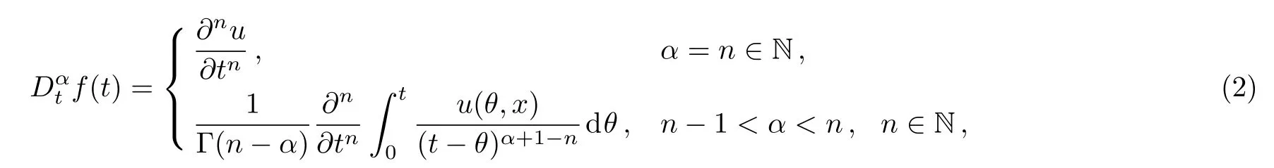
where Γ(z)is the Euler gamma function.

Assume that Eq.(1)is invariant under the one parameter Lie group of point transformations

whereεis the group parameter,and its associated Lie algebra is spanned by the following vector fields

Here

On the basis of the in finitesimal invariance criterion,one can get

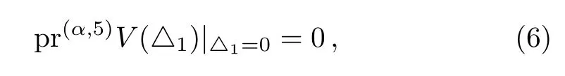
where

The prolongation operator pr(α,5)Vis

where

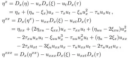
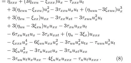
From Ref.[34],we have

and additional constraint condition is

Compared with the Lie symmetry method to integral order differential equations,one can see that constraint condition(9)and formula(11)are very important for the FDEs.

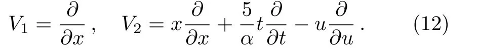
In the next section,by making use of the above discussion and Lie theory,we will study the F-G equation(1).Theorem 1The symmetry group of the equation is spanned by the following vector fields

ProofAssuming that Eq.(1)is invariant under the transformation group(3),one can get the symmetry equations as follows

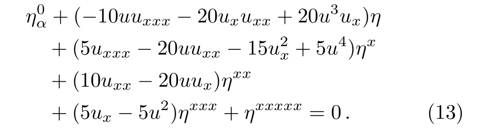
Substituting Eqs.(8)–(11)into Eq.(13),and letting all of the powers of derivatives ofuto zero,one can get

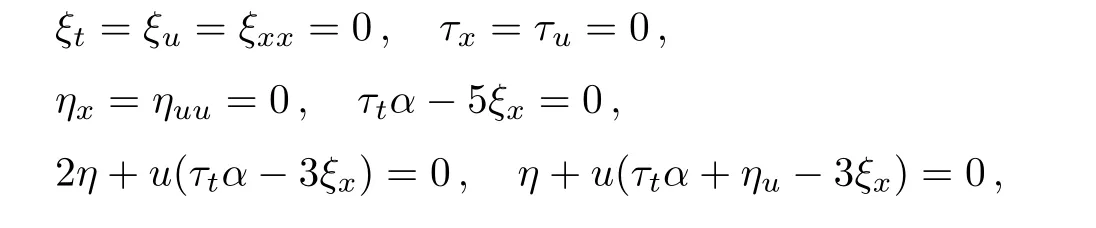
Solution of the above system gives

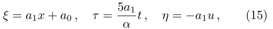
wherea1,a2are arbitrary constants.Thus the corresponding vector fields are

Then we have

which complete the proof.

3 Similarity Reductions

In this section,we applied the symmetries to construct similarity reductions for the time-fractional Fordy–Gibbons equation.

3.1 For the Symmetry V1

The invariant solutions are of the form

Substituting Eq.(18)into Eq.(1)yields the reduced fractional ODE

Then we obtain the invariant solution

for arbitrary constantc.

3.2 For the Symmetry V2

FromV2,we get the characteristic equation

Solving Eq.(21),we have the following similarity variables

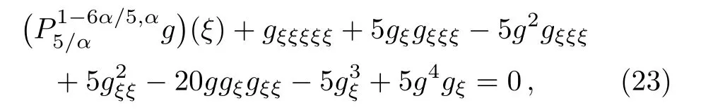
Theorem 2Under the transformation(22),Eq.(1)can be reduced to the following nonlinear ODE

with the Erd´elyi–Kober fractional differential operatorPτ,α

β

where

is the Erdlyi–Kober fractional integral operator.

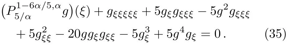
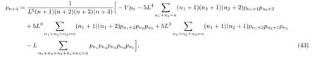
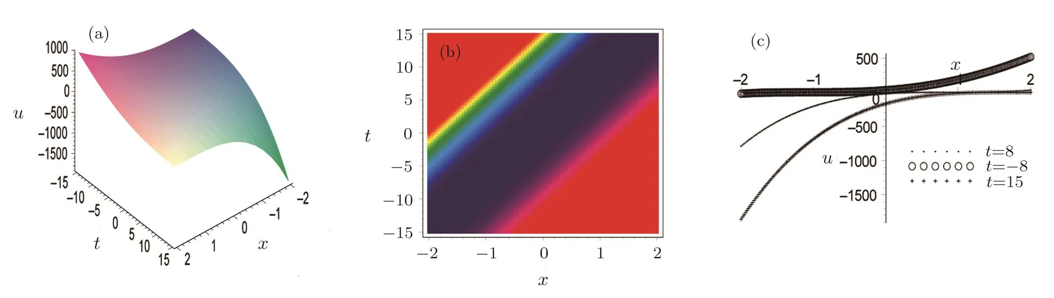
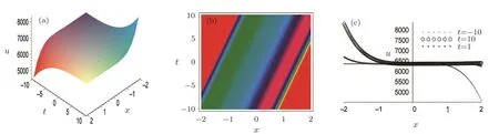
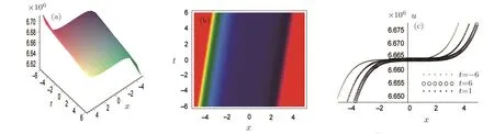
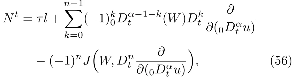
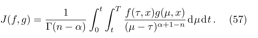
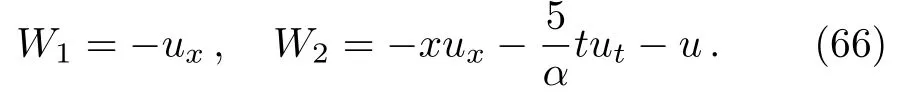
ProofFirstly we letn−1<α

Lettingv=t/s,one can get ds=−(t/v2)dv.Therefore,Eq.(27)can be rewritten as

Via the Erdlyi–Kober fractional integral operator(26),we can get

Taking advantage of the relation(ξ=xt−α/5),we can obtain

Therefore,one can get

Repeating the similar procedure as above forn−1 times,one has

Then using Eq.(24),we get

Substituting Eq.(33)into Eq.(29),we have

Hence,the time fractional Fordy–Gibbons equation can be reduced into the following ODE

This completes the proof.

4 Exact Power Series Solutions

Based on the power series method[35−37]and symbolic computations,[38−40]we will construct the exact power series solutions of Eq.(1).First we make use of a very important transformation

whereL,Vare arbitrary constants withL,V=0.Substituting Eq.(36)into Eq.(1),then we can obtain the following ODE

Integrating Eq.(37)with respect toξ,we can get

We suppose the solution of Eq.(38)as the following

wherepn(n=0,1,2,...)are constants. In view of Eq.(39),we have

Substituting Eqs.(39),(40)into Eq.(38),then one has

for alln=0,1,2,...

Whenn=0,from Eq.(41),we obtain

Whenn≥1,from Eq.(41),we obtain

Thus,the chosen constant numberspn(n=0,1,2,...)can be determined successively from Eqs.(42)and(43)in a unique manner.This implies that for Eq.(39),there exists a power series solution with the coefficients given by Eqs.(42)and(43).Furthermore,it is easy to prove the convergence of the power series(39)with the coefficients given Eqs.(42)and(43).Therefore,this power series solution(39)is an exact analytic solution.

Hence,the power series solution of Eq.(39)can be written as the following

wherep0,p1,p2,p3,L,Vare arbitrary constants,ξ=Lx+V tα/Γ(1+α),the other coefficientspn+4(n=0,1,2,...)are given by Eqs.(42)and(43)successively.

Fig.1 (Color online)Exact power series solutions u in system(44)for Eq.(1)by choosing suitable parameters(n=0):p0=p1=1,p2=2,p3=3,δ=0,k=2,λ=1,α =1,Γ =2,L=2,v=1.(a)Perspective view of the real part of exact power series solutions.(b)Overhead view of the solutions.(c)Wave propagation pattern of the x axis.

Fig.2 (Color online)Exact power series solutions u in system(44)for Eq.(1)by choosing suitable parameters(n=1):p0=p1=p2=p3=1,δ=1,k=3,λ=1,α =1,Γ =2,L=2,v=4.(a)Perspective view of the real part of exact power series solutions.(b)Overhead view of the solutions.(c)Wave propagation pattern of the x axis.

Fig.3 (Color online)Exact power series solutions u in system(44)for Eq.(1)by choosing suitable parameters(n=0):p0=2,p1=p2=1,p3=2,δ=1,k=2,λ=1,α =1,Γ =4,L=3,v=2.(a)Perspective view of the real part of exact power series solutions.(b)Overhead view of the solutions.(c)Wave propagation pattern of the x axis.

Fig.4 (Color online)Exact power series solutions u in system(44)for Eq.(1)by choosing suitable parameters(n=1):p0=2,p1=p2=p3=1,δ=0,k=3,λ=2,α =1,Γ =3,L=3,v=0.(a)Perspective view of the real part of exact power series solutions.(b)Overhead view of the solutions.(c)Wave propagation pattern of the x axis.

The graphical representation of the exact power series solutions are plotted in Figs.1–4.Figures 1 and 2 show the exact power series solutions ofuin system(44)whenn=0.Figures 3 and 4 show the exact power series solutions ofuin system(44)whenn=1.Furthermore,Fig.1(a)shows the three-dimensional space graphic whenx=−2,...,2,t=−15,...,15.Figure 1(b)shows the density graphic whenx=−2,...,2,t=−15,...,15.Figure 1(c)shows the wave propagation pattern of thexaxis whenp0=p1=1,p2=2,p3=3,δ=0,k=2,λ=1,α=1,Γ=2,L=2,v=1,x=−2,...,2.Figures 2–4 take the same values of as Fig.1,and have the same representation.

5 Conservation Laws of FFG Equation

In this section,on the basis of Eq.(12),we will construct conservation laws for the time-fractional Fordy–Gibbons equation.Similar to the definition of conserved vector for integer order PDEs,a vectorC=(Ct,Cx)is called a conserved vector for Eq.(1)a conserved vector satisfies the following conservation equation

whereCt=Ct(t,x,u,...),Cx=Cx(t,x,u,...).Equation(45)is called a conservation law for Eq.(1).

A formal Lagrangian for Eq.(1)can be written in the following form

Here,v(x,t)is a new dependent variable.Due to the formal Lagrangian,an action integral is given by

The Euler–Lagrange operator is defined by

whereis the adjoint operator ofFor the Riemann–Liouville fractional differential operators,we have the form

where

is the right-sided fractional integral of ordern−αandis the right-sided Caputo operator of fractional differentiation of orderα.

With the Riemann–Liouville fractional derivative,Eq.(1)can be rewritten in the form of conservation law form(45)as

The adjoint equation is similarly to the case of integerorder nonlinear differential equations.So we have adjoint equation to the nonlinear equation(1)as Euler–Lagrange equation

Taking into account the case of the variablest,x,andu(x,t),we have

wherelis the identity operator,δ/δushows the Euler-Lagrange operator,NtandNxare the Noether operators,is given by

When Riemann–Liouville time-fractional derivative is used in Eq.(1),the operatorNtis given by

whereJis the integral

Then,the operatorNxis defined by

For any operatorXof Eq.(1)and its any solutions,we have

This equality yields the conservation law

From above,we have two kinds of conservation laws as follows.

Case 1Whenα∈(0,1),for the case,using Eqs.(56)and(58),one can get the components of conserved vectors

wherei=1,2 and functionsWiare

Case 2Whenα∈(1,2),for the case,we get the components of conserved vectors

wherei=1,2 and functionsWihave the form

6 Conclusion and Discussions

In this paper,we applied Lie symmetries to study the time-fractional Fordy–Gibbons equation with Riemann–Liouville derivative.Based on the Lie symmetries we derived,symmetry reductions,exact power series solutions and conservation laws are obtained.However,the study of symmetry properties of FDEs is just at the start stage and there is still much work to be considered in depth.In conclusion,the symmetry analysis which based on the Lie group method is a very useful method and is worthy of investigate further.

[1]R.Hilfer,Applications of Fractional Calculus in Physics,World Scientific,Singapore(2000).

[2]A.A.Kilbas,H.M.Srivastaa,and J.J.Trujillo,Theory and Applications of Fractional differential Equations,The Netherlands,Amsterdam(2006).

[3]J.Sabatier,O.P.Agrawal,and J.A.Tenreiro Machado,Advances in Fractional Calculus,Theoretical Developments and Applications in Physics and Engineering,Springer,Berlin(2007).

[4]L.V.Ovsiannikov,Group Analysis of differential Equations,Academic Press,New York(1982).

[5]P.J.Olver,Application of Lie Group to differential Equation,Springer,New York(1986).

[6]G.W.Bluman and S.Kumei,Symmetries and differential Equations,Springer,New York(1989).

[7]N.H.Ibragimov,Lie Group Analysis of differential Equations-Symmetries,Exact Solutions and Conservation Laws,Florida,CRC(1994).

[8]S.Y.Lou,Z.Naturforsch.53a(1998)251;H.C.Hu,and S.Y.Lou,Z.Naturforsch.A 59(2004)337;X.P.Cheng,C.L.Chen,and S.Y.Lou,Wave Motion 51(2014)1298;S.Y.Lou,Stud.Appl.Math.134(2015)372.

[9]Y.Chen,Z.Y.Yan,B.Li,and H.Q.Zhang,Commun.Theor.Phys.38(2002)261;X.R.Hu and Y.Chen,Commun.Theor.Phys.53(2010)803.

[10]Z.Y.Yan,Appl.Math.Lett.47(2015)61;B.Li,Y.Q.Li,and Y.Chen,Commun.Theor.Phys.51(2009)773.

[11]C.Z.Qu,S.F.Shen,and S.L.Zhang,AIP Conf.Proc.1212(2010)219.

[12]S.L.Zhang,S.Y.Lou,and C.Z.Qu,J.Phys.A:Math.Gen.36(2003)12223.

[13]G.W.Bluman,S.F.Tian,and Z.Z.Yang,J.Eng.Math.84(2014)87.

[14]S.F.Tian,Y.F.Zhang,B.L.Feng,and H.Q.Zhang,Chinese Ann.Math.36B(2015)543.

[15]S.F.Tian,T.T.Zhang,P.L.Ma,and X.Y.Zhang,J.Nonlinear Math.Phys.22(2)(2015)180.

[16]R.K.Gazizov,A.A.Kasatkin,and S.Y.Lukashchuk,Vestnik USATU 9(2007)125.

[17]R.K.Gazizov,A.A.Kasatkin,and S.Y.Lukashchuk,Phys.Scr.2009(2009)014016.

[18]R.Sahadevan and T.Bakkyaraj,J.Math.Anal.Appl.393(2012)341.

[19]G.W.Wang and T.Z.Xu,Nonlinear Dyn.76(2014)571.

[20]Q.Huang and R.Zhdanov,Physica A 409(2014)110.

[21]S.Y.Lukashchuk and A.V.Makunin,Appl.Math.Comput.257(2015)335.

[22]E.Noether,Transp.Theory Stat.Phys.1(1971)186.

[23]G.S.F.Frederico and D.F.M.Torres,J.Math.Anal.Appl.334(2007)834.

[24]T.M.Atanackovic,S.Konjik,S.Pilipovic,and S.Simic,Nonlinear Anal.71(2009)1504.

[25]A.B.Malinowska,Appl.Math.Lett.25(2012)1941.

[26]T.Odzijewicz,A.B.Malinowska,and D.F.M.Torres,Cent.Eur.J.Phys.11(2013)691.

[27]L.Bourdin,J.Cresson,and I.Gre ff,Commun.Nonlinear Sci.Numer.Simul.18(2013)878.

[28]N.H.Ibragimov,J.Math.Anal.Appl.333(2007)311.

[29]S.Y.Lukashchuk,Nonlinear Dyn.80(2015)791.

[30]A.P.Fordy and J.Gibbons,Phys.Lett.A 75(1980)325.

[31]N.A.Kudryashov and M.V.Demina,Phys.Lett.A 363(2007)346.

[32]F.Mainardi,Fractional Calculus and Waves in Linear Viscoelasticity,World Scientific,Singapore(2010).

[33]I.Podlubny,Fractionl differential Equations:An Introduction to Fractional Derivatives,Fractional differential Equations,to Methods of Their Solution and Some of Their Applications,Academic press,New York(1998).

[34]R.K.Gazizov,A.A.Kasatkin,and S.Y.Lukashchuk,Phys.Scr.136(2009)014016.

[35]R.Sahadevan and T.Bakkyaraj,J.Math.Anal.Appl.393(2012)341.

[36]V.A.Galaktionov and S.R.Svirshchevskii,Exact Solutions and Invariant Subspaces of Nonlinear Partial Dif-ferential Equations in Mechanics and Physics,Chapman and Hall/CRC,Boca Raton,Florida(2006).

[37]N.H.Asmar,Partial differential Equations with Fourier Series and Boundary Value Problems,2nd ed.China Machine Press,Beijing(2005).

[38]S.F.Tian,F.B.Zhou,S.W.Zhou,and T.T.Zhang,Modern Phys.Lett.B 30(2016)1650100;S.F.Tian and H.Q.Zhang,J.Math.Anal.Appl.371(2010)585;S.F.Tian and H.Q.Zhang,Chaos,Solitons&Fractals 47(2013)27.

[39]S.F.Tian and H.Q.Zhang,J.Phys.A:Math.Theor.45(2012)055203;S.F.Tian and H.Q.Zhang,Stud.Appl.Math.132(2014)212.

[40]C.Q.Dai and Y.Y.Wang,Nonlinear Dyn.83(2016)2453;C.Q.Dai,Y.Wang,and J.Liu,Nonlinear Dyn.84(2016)1157;C.Q.Dai and Y.J.Xu,Appl.Math.Model.39(2015)7420.