High Order Numerical Methods for LESof Turbulent Flows with Shocks

D.V. Kotov, H.C. Yee, A. Wray, A. Hadjadj, B. Sjögreen

(1. Center for Turbulence Research, Stanford University, Stanford, CA 94305, USA 2. NASA Ames Research Center, Moffett Field, CA 94035, USA 3. CORIA UMR 6614 & INSA de Rouen, 76800 St-Etienne du Rouvray, France 4. Lawrence Livermore National Laboratory, Box 808, L-422, Livermore, CA 94551, USA)



High Order Numerical Methods for LESof Turbulent Flows with Shocks

D.V. Kotov1, H.C. Yee2,*, A. Wray2, A. Hadjadj3, B. Sjögreen4

(1. Center for Turbulence Research, Stanford University, Stanford, CA 94305, USA 2. NASA Ames Research Center, Moffett Field, CA 94035, USA 3. CORIA UMR 6614 & INSA de Rouen, 76800 St-Etienne du Rouvray, France 4. Lawrence Livermore National Laboratory, Box 808, L-422, Livermore, CA 94551, USA)

Simulation of turbulent flows with shocks employing subgrid-scale (SGS) filtering may encounter a loss of accuracy in the vicinity of a shock. This paper addresses the accuracy improvement of LES of turbulent flows in two ways: (a) from the SGS model standpoint and (b) from the numerical method improvement standpoint. The high order low dissipative method of Yee & Sjögreen (2009) using adaptive flow sensors to control the amount of numerical dissipation where needed is used for the LES simulation. The considered improved dynamics model approaches include applying the one-sided SGS test filter of Sagaut & Germano (2005) and/or disabling the SGS terms at the shock location. For Mach 1.5 and 3 canonical shock-turbulence interaction problems both of these new approaches show a similar accuracy improvement to that of the full use of the SGS terms. One of the numerical accuracy improvements included here applies Harten’s subcellre solution procedure to locate and sharpen the shock, and uses a one-sided test filter at the grid points adjacent to the exact shock location.

High order low dissipative scheme, Germano model, LES filtering, DNS, Subcell resolution scheme, Shock/turbulence interaction

0 Introduction

The presence of a shock wave in turbulent flows might cause a numerical accuracy problem in employ-ing the subgrid-scale (SGS) filtered equations across shocks, depending on the large eddy simulation (LES) model, the grid size, as well as the shock strength. Since the majority of dynamic LES models involve filter operations, hereafter referred to as “LES filters” to distinguish them from standard

“numerical filters for numerical method develop-ment”, when the LES filtered equations are applied through the shock, the Rankine-Hugoniot relations are affected by the filtering operation, since the filtered variables are not discontinuous.In the present study we consider LES employing the dynamic Germano procedure [1] for calculating the model coefficients. The dynamic Germano procedure was developed for shock free turbulence. Sagaut and Germano [2] have noticed that the usual filtering procedures, based on a central SGS spatial filter that provides information from both sides, when applied around the shock, produce parasitic contributions that affect the filtered quantities. They suggested using non-centered SGS filters to avoid this nonphysical effect.In Grube & Martin [3] shock-confining filters have been proposed instead. Another approach based on the deconvolution method is considered in Adams & Stolz [4].

Aside from the subgrid scale filtering procedure, the accuracy of direct numerical simulation (DNS) and LES with shocks depends heavily on the accuracy of the numerical scheme. For the last decade high order shock-capturing methods with numerical dissipation controls have been the state-of-the-art numerical approach for DNS and LES of turbulent flows with shocks. See, for example, [5-15]. The majority of these methods involve flow sensors with parameter tuning applied depending on the flow type. Some of the flow sensors were designed for certain flow types and might not preserve their high accuracy when used to simulate a different flow type. In a study presented in Johnsen et al.

[13], all of the shock-capturing schemes involve tuning of parameters. It appears that the Yee & Sjogreen filter scheme is not as accurate as the hybrid scheme presented in [13] as the key parameter κ responsible for minimizing the numerical dissipation in the 2007 Yee & Sjogreen scheme [6] was mandated to be the same for all considered test cases reported in [13]. See [5, 10] for a description of better control of numerical dissipation using an adaptive localκ. The hybrid scheme presented in [13] which employed the Ducros et al. flow sensor [16] also consists of a key tuning parameterδ. From our study presented in [17] of the same Taylor-Green vortex problem considered in [13], the cut-off parameterδshould be set to 1 to achieve the best accurate result. On the other hand, for the isotropic turbulence with shocklets test case, the Ducros et al. flow sensorδparameter has to be reduced, mostly by trial and error. Yet in another study [11] for turbulence interacting with a high speed stationary shock, depending on the Mach number and turbulent Mach number, a differentδis required for each case. It is noted that for LES simulation it is more important to use low-dissipative schemes as added dissipation has already introduced by the SGS model.

Objective: In recognizing the different requirements on numerical dissipation control for DNS and LES of a variety of compressible flow types, Yee & Sjogreen [5] presented a general framework for a localκand the accompanying variety of flow sensors were introduced into their high order nonlinear filter scheme.Aside from suggesting different localκformulation, Yee & Sjogreen also proposed the use of a combination of different flow sensors. Their proposed scheme with numerical dissipation control had not been studied extensively until recently. A subset to the sequel to [5] was presented in [10, 17-19].

This low dissipative high order nonlinear filter scheme [5] has recently been employed for DNS and LES computations [17,20] to capture the global turbulence flow accurately for shock-free flows, low speed flows with shocklets and problems containing strong shock waves. Previous studies [21, 22] indicated that the combination of the nonlinear filter scheme with Harten’s subcell resolution method [23] is able to improve the accuracy (reduce the dissipation) near the shock within a grid cell, especially for stiff reacting flows. This high order nonlinear filter scheme is used for the present DNS and LES studies. The considered approaches include applying a one-sided SGS test filter [2] and/or disabling of the SGS terms at the shock location. The test problems considered are the Mach 1.5 and 3 canonical shock-turbulence interaction flows. We consider the improvement of our high order nonlinear filter scheme for LES with strong shock by employing Harten’s subcell resolution procedure to locate and sharpen the shock.

Outline: The outline of the paper is as follows. Section 1 provides a description of the LES model considered and the numerical scheme used to solve the governing equations with the details on the three modifications of the LES filtering procedure. Section 2 describes the shock-turbulence interaction problem setup and a comparison of the the current DNS computations with the digitized results from [24]. Then LES computations employing the high order nonlinear filter numerical method are compared with the filtered DNS data, and with LES results using standard and modified SGS LES filtering procedures.

1 Mathematical Formulation and Numerical Methods

1.1 Governing Equations and LES Model

We consider the filtered compressible Navier-Stokes equations written in the conservative form gives:

(1)

(2)

(3)

(4)

(5)

(6)

(7)

(8)

(9)

(10)

where

(11)

(12)

(13)

and〈f〉Hstands for averaging in homogeneous (periodic) directions.

For the considered test case with low turbulent Mach numberMt<0.4 it is shown [26] that the isotropic part of the SGS stress can be neglected:CI=0. The Germano procedure requires an explicit test filtering operation, denoted here with the hat symbol. For the Germano procedure we use a 3D filtering operator based on a 1D trapezoidal filter:

(14)

Note that according to [27] the width of the discrete filter can be estimated as

(15)

1.2 High-Order Filter Schemes

This section gives a brief overview of the high order nonlinear filter scheme of Yee et al. [5, 6, 8, 18] for accurate computations of DNS and LES of compressible turbulence for a wide range of flow types. With in the confines of the considered integrated approach, this method attempt to introduce as little numerical dissipation as possible. The basic design principle of the filter scheme is to minimize the use of numerical dissipation inherited from standard high order shock-capturing schemes that were developed for rapidly developing unsteady shock flows. Without any modification or redesigning of these standard schemes, they are too diffusive for DNS and LES computations. The nonlinear filter scheme consists of three steps, as described in the following three subsections.

1.2.1 Preprocessing Step

Before the application of a high order non-dissipative spatial base scheme, a preprocessing step is employed to improve numerical stability. The inviscid flux derivatives of the governing equations are split into the following three ways, depending on the flow types and the desire for rigorous mathematical analysis or physical argument.

· Entropy splitting of [28-30]. This splitting of the inviscid flux derivative into two parts is non-conservative and the derivation is based on the entropy variables and energy norm stability for the compressible Euler equations with boundary closure for the initial boundary value problem.

· The Ducros et al. splitting [31] for systems. This is a conservative splitting and the derivation is based on physical arguments.

· Tadmor entropy conservation formulation for systems [32]. The derivation is based on mathe-matical analysis. It is a generalization of Tadmor’s entropy formulation to systems and has only been tested on a limited number of test cases. The findings are that the Tadmor entropy conservation formulation is more diffusive than the other two splittings.

1.2.2 Base Scheme Step

A full time step is advanced using a high order non-dissipative (or very low dissipation) spatially central scheme on the split form of the governing partial differential equations (PDEs) (i.e., after the preprocessing step). A summation-by-parts (SBP) boundary operator [33, 34] and matching order conservative high order free stream metric evaluation for curvilinear grids [35] are used. Note that the base scheme can be any high order standard central scheme, compact scheme [36], or spectral method. However, the same entropy stable SBP boundary closure for high order central schemes is not valid for the latter two base schemes.

High order temporal discretization such as the third-order or fourth-order Runge-Kutta (RK3 or RK4)method is used. It is remarked that other temporal discretizations can be used for the base scheme step.

1.2.3 Post-Processing (Nonlinear Filter Step)

To further improve the accuracy of the computed solution from the base scheme step, after a full time step of a non-dissipative high order spatial base scheme on the split form of the governing equation(s), the post-processing step is used to nonlinearly filter the solution by a dissipative portion of a high order shock-capturing scheme with a local flow sensor. The flow sensor provides locations and amounts of built-in shock-capturing dissipation that can be further reduced or eliminated locally. At each grid point a local flow sensor is employed to analyze the regularity of the computed flow data. Only the strong discontinuity locations would receive the full amount of shock-capturing dissipation. In smooth regions no shock-capturing dissipation would be added, unless high frequency oscillations are developed. This is due to the possibility of numerical instability in long time integrations of nonlinear governing PDEs. In regions with strong turbulence, if needed, a small fraction of the shock-capturing dissipation would be added to improve stability.

Note that the filter numerical fluxes only involve the inviscid flux derivatives, regardless if the flow is viscous or inviscid. If viscous terms are present, a matching high order central difference operator (as the inviscid difference operator) is included on the base scheme step. For ease of SBP numerical boundary closure for the viscous flux derivatives, the same inviscid central difference operator for the first derivativeis employed twice for the viscous flux derivatives.

LetU*be the solution after the completion of the full time step of the base scheme step. The final update of the solution after the filter step is (with the numerical fluxes in they- andz-directions suppressed as well as their correspondingy- andz-direction indices on thexinviscid flux suppressed)

(16)

(17)

(18)

Hereuis the velocity vector,ωis the vorticity magnitude andεis a small number to avoid division by zero (e.g., 10-6). The Ducros et al. flow sensor consists of a cut off parameterδthat can be used to switch on or off the dissipative portion of the high order shock-capturing scheme. Ifδis set to be one, the dissipation only switches on when it encounters a shock wave. For a lower value of the cut offδparameter, vorticity can be detected.

It is noted that the nonlinear filter step described above should not be confused with the LES filtering operation. For previous studies on the performance of this filter scheme in DNS and LES simulations, see[5, 7-9, 18, 37-39]. This scheme has been validated for DNS of a 3D channel flow, 2D temporal and spatial evolving mixing layers, Richtmyer-Meshkov instability, 3D Taylor-Green vortex, 3D isotropic turbulence with shocklets, extreme condition flows, and a 3D supersonic LES of temporal evolving mixing layers by comparing with experimental data.

1.3 Modifications of the LES Filtering Procedure for Flows with Shocks

During LES computation using the filtered governing equations, there are two additional sources of inaccuracy that may appear near the shock. The first one is connected with the numerical scheme used for solving the governing equations. Away from the shock the high order central scheme is applied, introducing a negligible amount of numerical dissipation. However, in the vicinity of the shock the shock-capturing scheme is activated, introducing numerical dissipation into the computed solutions. The amount of numerical dissipation introduced by the shock capturing scheme, if not controlled correctly, may be higher than the turbulent dissipation modeled by the SGS terms (depending on the particular problem parameters). Hadjadj and Barmeo [40, 41] proposed to locally disable the SGS terms in order to obtain more accurate results. Denote this procedure as LES-Z:

Procedure LES-Z

1)Employflowsensortodetectshocks

2)ObtainCSfromDynamicGermanoProcedureexceptneartheshock

3)SetCS=0withingridstencilwidthoftheschemeatshock

SettingCS=0 within the grid stencil width of the shock location (according to the computed flow sensor indicator) might appear to be too abrupt. An alternate procedure would be to setCS=0 at the shock location with a smooth transition functionCSsuch astanhin the vicinity of the shock. Our studies show that settingCS=0 for the whole WENO grid stencil width rather than atanhsmoothing function produces better results.

The second additional source of inaccuracy of LES results in the vicinity of the shock comes from the fact that the explicit filtering operation in (10)-(13) is applied across the shock, causing inaccuracy of the results. In this case, as is pointed out in Sagaut & Germano [2], a one-sided filtering operation should be used instead of a central form. Denote this procedure as LES-1S:

Procedure LES-1S

1)Employflowsensortodetectshocks

2)ObtainCSfromDynamicGermanoProcedureexceptneartheshock

3)Applyone-sidedSGSfilteringprocedureof[2]totheleftandrightoftheshocklocation

ThethirdconsideredmodificationisbasedonHarten’ssubcellresolution(SR)approach[23]combinedwithENOreconstruction.Anyshock-capturingmethodappliedattheshockwillresultinsmearingtheshock.ByestimatingtheexactshocklocationthroughSRandusingENOreconstructiononecansharpentheshocksothatthenumericaldissipationisminimizedmorelocally.DenotethisLESprocedureasSR:

ProcedureLES-Z-SRandLES-1S-SR

1)Employ flow sensor to detect shocks

2) Employ Harten’s SR approach to confine shock location within two grid cells

3) Employ ENO reconstruction to improve the solution points adjacent to the shock

4) Obtain CSfrom Dynamic Germano Procedure except near the shock

5) (a) Set CS=0 within grid stencil width of the scheme at shock (denoted by LES-Z-SR) or (b) Apply one-sided SGS filtering procedure of [2] to the left and right of the shock location (denoted by LES-1S-SR).Note that the SR procedures here is apply to the conservative variables. They are NOT applied the modified numerical flux as indicated in Shu & Osher [42] for RK methods

2 3D Turbulence Across a Supersonic Shock Wave

2.1 Problem Setup

The 3D test case considered here concerns an initial turbulence disturbance at the inflow boundary interacting with a stationary supersonic planar shock wave. The problem has been studied by previous investigators,mainly related to DNS computations; see e.g. [24, 41, 43]. Here we choose the configuration considered in the DNS study of [24]. Fig.1 shows a schematic of the problem setup. The computational domain is -2≤x≤-2+4π, 0≤y≤2π and 0≤z≤2π. The grid is uniform in all directions with the spacing inxseveral times finer than inyandz(see [24] for explanation). We solve the filtered governing Eqs.(1)- (3) in a non-dimensional form. The Yee et al. filter scheme with Ducros et al. flow sensor[16] is used for integration of the Ducros et al.

[31] splitted form of the governing equations. The spatial base scheme is the eighth-order central differencing and the nonlinear filter scheme is the dissipative portion of the seventh-order WENO scheme (WENO7). This nonlinear filter scheme, including the Ducros et al. splitting of the governing equation, is denoted by WENO7fi + split (or WENO7fi for ease of discussion). Since the initial data consists of a planar shock in thex-direction, numerical dissipation should be mainly needed in thex-direction. In order to obtain more accurate results, WENO dissipation is employed only in thexdirection at the postprocessing stage of the Yee et al. filter. The inflow and outflow boundary conditions are applied in the streamwise direction and periodic boundary conditions are applied in the transverse directions.

Outflow boundary condition. In order to avoid acoustic reflections of subsonic flow from the outflow boundary a non-reflective sponge layer is employed on the region near the outflow. The length of this layer isxmax-xsp=π. The sponge layer is implemented by introducing the following source term into the Eqs. (1)- (3):

(19)

wheref=ρ，ρui，ρEand 〈·〉yzdenotes averaging in they- andz-directions.

The outflow pressurep∞is chosen such that the mean shock location is stationary. For laminar flow Rankine-Hugoniot conditions give

(20)

wherep0is the inflow mean pressure,u0is the mean inflow velocity,c0is the mean inflow speed of sound andUSis the shock velocity. As the inflow condition is turbulent, the Rankine-Hugoniot conditions are valid only instantaneously but not in average. After an initial guess based on (20) the outflow pressure is refined by an iteration procedure, integrating the governing equations on a coarse grid and updating the pressure according to the formula

(21)

See [24] for more details.

Gathering statistics. The simulation statistics for a given functionfare obtained by averaging in time and in homogeneous directions:

(22)

whereLyandLzare domain sizes in transverse directions. The averaging is performed over a time span Δt≈100/(κ0u0).ConvergenceisconfirmedbycomparingtheresultswithstatisticsobtainedovertimespanΔt/2. The statistics are gathered after the transient period has passed. Transient timet0is estimated ast0≫Lx/u0, whereLxis the domain size in the streamwise direction. The correct choice of transient time is confirmed by comparing with the statistics obtained starting from timet0/2.

Fig.1 Turbulence across a shock wave problem setup.

(a)

(b)Fig.2 DNS on grid of 1553×2562points by WENO7fi,M= 1.5: Instantaneous velocity field ux (a)and uy (b), slice z=const.

2.2 DNS Comparison

2.2.1 Comparison with Work of Larsson [24] and Standard WENO Schemes

The instantaneous streamwise and transverse velocity fields are shown in Fig.2 using WENO7fi+split.For ease of reference, hereafter, WENO7fi means WENO7fi+split. During the computation over a long time evolution, the shock slightly moved upstream. For the case with the given turbulent Mach numberMt=0.16, the shock is wrinkled due to turbulent inflow. As shown in previous studies [24, 43], the shock may break at higher turbulent Mach numbersMt. The turbulence is compressed by the shock, and immediately behind the shock it is anisotropic. The comparison of turbulent statistics for streamwise and transverse components of the vorticity and Reynolds stress shows that the turbulence becomes isotropic again downstream ofx≈3(figure not shown). Downstream ofx=8 turbulence is essentially damped with the sponge source term.

Figs.3-8 represent the DNS statistics for differnet cases. The averaging operation is performed in transverse directions and in time. The averages are collected after the initial transition disappears. The averaging time period ist=100/(κ0u0). The plots are presented in the reference frame of the average shock location.

The comparison between the DNS statistics obtained in this work using the ADPDIS3D [6] code and the data obtained from digitizing the solution [24] is shown in Fig. 3. The results obtained in both of these works are in good agreement. The grid resolution in the vicinity of the shock is the same. In Larsson & Lele [24] grid clustering near the shock has been employed, resulting in a smaller grid size, 694×2562. The work [24] employs the HYBRID code, which also uses a Ducros et al. flow sensor for shock detection. However, in Larsson & Lele [24] WENO dissipation has been introduced at every Runge-Kutta stage, whereas the Yee et al. scheme allows decreasing the computational cost by employing WENO dissipation only after the full Runge-Kutta step.

The comparison between the filtered DNS data and the results obtained with different numerical schemes on the coarse grid with 389×642points is shown in Fig.4. Here we compare the results obtained by the fifth-order WENO (WENO5) and WENO7 with the results obtained by the filter counterpart of WENO7 with Ducros et al. splitting of the governing equations (WENO7fi+split). The comparison of WENO5,WENO7 and WENO7fi+split is shown in Fig.4. For Fig.4, each of the considered schemes is employed in all three directions. Solution by WENO7fi is closer to the filtered DNS solution than WENO5 and WENO7.WENO5 is far too dissipative for DNS computation with this coarse grid.

2.2.2 DNS Grid Refinement Study

Since the peak values of the Reynolds stress in the streamwise direction for the medium and fine grid(777×1282and 1553×2562) in our preliminary study [20] are not quite converged, in order to confirm the proper grid size for the DNS solution to be used as a reference solution for our LES comparison, a five-level DNS grid refinement is performed forM=1.5. The five grids are the original three grids together with two finer grids of 2329×2562and 2329×3842. For theM=3 case, a smaller time step has to be used for stability considerations. Due to the higher CPU time required forM=3, only one added grid refinement(2329×2562) over our earlier work is performed.

The results of the added level grid refinement study for casesM=1.5 andM=3 are shown in Figs.5-9. Figs. 6 and 9 show the close up peak solutions at the shock location for the grid refinement comparison. The last two finer grid solutions are very close forM=1.5. ForM=3 a finer grid is needed to obtain a converged peak solution near the shock.

Fig.3 DNS comparison (WENO7fi vs. Hybrid WENO7): WENO7fi solution uses data obtained from digitizing the solution from [24] employing the HYBRID method. Top row: streamwise (left) and transverse(right) Reynolds stress components. Bottom row: streamwise (left) and transverse (right) vorticity components.

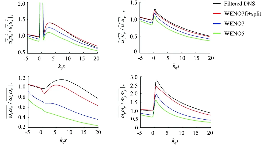
Fig.4 DNS, WENO5, WENO7 and WENO7fi method comparison: Comparison to filtered DNS data ofthe statistics obtained by the different numerical schemes on a coarse grid 389×642, M=1.5. Top row:streamwise (left) and transverse (right) Reynolds stress components. Bottom row: streamwise (left) and transverse (right) vorticity components.

Fig.5 DNS, WENO7fi, M=1.5: Five-level DNS grid refinement study on grids with 389×642, 777×1282, 1553×2562, 2329×2562 and 2329×3842 points. Top row: streamwise (left) and transverse (right) Reynolds stress components. Bottom row: streamwise (left) and transverse (right) vorticity components.

Fig.6 DNS, WENO7fi, M=1.5, zoom in the vicinity of the shock: Five-level DNS grid refinement study on grids with 389×642, 777×1282, 1553×2562, 2329×2562 and 2329×3842points. Top row: streamwise(left) and transverse (right) Reynolds stress components. Bottom row: streamwise (left) and transverse (right) vorticity components.

Fig.7 DNS, WENO7fi, M=1.5, peak streamwise Reynolds stress component in the vicinity of the shock: Five-level DNS grid refinement study on grids with 389×642, 777×1282,1553×2562, 2329×2562 and 2329×3842points.

2.2.3 Spectra of the DNS Grid Refinement Study

The spectra of the DNS grid refinement study are shown in Figs. 11 and 12. All the plots correspond to the planex= 0 which is slightly behind the shock location. The spectra for all the grids match at the inertial range, while showing typical dependence on the grid resolution in the dissipation range. The analysis of spectra obtained on a grid 389×642confirms the validity of applying LES modeling even to this low-resolution grid.

In conclusion, the present DNS refined study indicated that the 1553×2562grid forM=1.5 can be used as a DNS reference solution for our LES study.

2.3 LES Filters Comparison

In this section we compare the results obtained by the Germano model using different filtering procedures (LES with the original SGS filtering procedure, LES-Z, LES-1S and LES-SR) with the DNS solution filtered to the size of the LES grid. The comparison of the original LES SGS model using WENO7fi with LES-Z and LES-1S by WENO7 (LES-Z/WENO7 and LES-1S/WENO7) is shown in Fig.13. From this comparison the low dissipative property of WENO7fi using the original LES SGS model exhibits higher accuracy than the results with the LES-Z/WENO7 or LES-1S/WENO7.

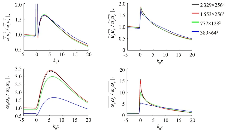
Fig.8 DNS, WENO7fi, M=3: Four-level DNS grid refinement study on grids with 389×642, 777×1282,1553 ×2562and 2329×2562points. Top row: streamwise (left) and transverse (right) Reynolds stress components. Bottom row: streamwise (left) and transverse (right) vorticity components.

Fig.9 DNS, WENO7fi, M=3, zoom in the vicinity of the shock: Four-level DNS grid refinement study on grids with 389 ×642, 777×1282, 1553×2562and 2329×2562points. Top row: streamwise (left) and transverse (right)Reynolds stress components. Bottom row: streamwise (left) and transverse (right) vorticity components.

The comparison between the different SGS modifications using WENO7fi on a grid with 389×642points for the caseM=1.5 is shown in Figs. 14 and 15. In the considered case the results obtained using LES-Z and LES-1S are closer to the filtered DNS than standard LES. LES-1S performs slightly better than LES-Z. The reasons for the small improvement between LES and the two improved SGS models might be due to WENO7fi’s good control of numerical dissipation and the fact that it is near the implicit LES limit for even this coarse gird case. In addition, one can observe that the coarse DNS (no LES) solution is under-resolved.However, the difference between LES-1S and LES-Z may be more significant for other flow conditions, e.g.,higher Mach and turbulent Mach numbers.

Fig.10 DNS, WENO7fi, M=3, peak streamwise Reynolds stress component in the vicinity of the shock: Four-level DNS grid refinement study on grids with 389 ×642, 777×1282, 1553×2562and 2329 ×2562 points.

The results for the same case on a two times finer grid (777×1282) can be found in [45]. All results obtained on this grid are quite close to each other. However, on this grid LES without any modification of the filtering procedure is slightly closer to the filtered DNS data. One can assume that the shock is resolved enough at this level of grid refinement so that there is no need for additional shock treatment.

Fig.11 DNS, WENO7fi, M=1.5, velocity spectrum,slice at x=0: Five-level DNS grid refinement study on grids with 389×642, 777×1282, 1553×2562, 2329×2562and 2329×3842points.

Fig.12 DNS, WENO7fi, M=3, velocity spectrum, slice at x=0: Four-level DNS grid refinement study on grids with 389×642, 777 ×1282, 1553×2562and 2329×2562points.

Fig.13 LES, WENO7 vs. WENO7fi, M=1.5: Comparison to filtered DNS data of the statistics obtained by LES with WENO7 and WENO7fi for different filtering procedures (LES-Z, and LES-1S) on grid 389×642. Top row: streamwise (left) and transverse (right) Reynolds stress components. Bottom row:streamwise (left) and transverse (right) vorticity components.

Fig.14 LES, WENO7fi, M=1.5: Comparison to filtered DNS data of the statistics obtained by LES with different filtering procedures (original SGS LES, LES-Z, and LES-1S) on grid 389×642. Top row:streamwise (left) and transverse (right) Reynolds stress components. Bottom row: streamwise (left) and transverse (right) vorticity components.

Fig.15 LES, WENO7fi, M=1.5, zoom in the vicinity of the shock: Comparison to filtered DNS data of the statistics obtained by LES with different filtering procedures (original SGS LES, LES-Z, and LES-1S) on grid 389×642. Top row: streamwise (left) and transverse (right) Reynolds stress components. Bottomrow: streamwise (left) and transverse (right) vorticity components.

A similar comparison of the methods on the grid with 389×642 points for the higher Mach number case (M=3) can be found in [45]. The behavior of the methods is similar to theM=1.5 case, but LES-Z performs slightly better in this case than LES-1S. The difference is more noticeable in the plot for the transverse vorticity component.

Figures 16 and 17 show the comparison of LES-Z, LES-1S with LES-Z-SR and LES-1S-SR. The SR procedure only increases the accuracy in certain flow variables over the no SR case. As originally expected, LES using the SR procedure helps improve the accuracy in the vicinity of the shock. A

careful examination at the finer DNS grids presented earlier shows that the 4 peak values by SR indicate improved accuracy over the no SR case. The simplified SR procedures might be a contributing factor to the lack of bigger accuracy improvement over the no SR procedure. It appears that the proposed LES using the SR model needs further refined consideration.

2.3.1 Comparison of Spectra of Different LES Filter Procedures

The spectrum of the LES with different filtering procedures on a grid with 389×642points for the caseM=1.5 at slicex=0 is shown in Fig.19. All LES spectra are in a good agreement with the filtered DNS spectrum obtained on a grid with 2329×3842points. The analysis shows that the LES spectrum is not affected by the employment of filtering procedures considered above.

Fig.16 LES, WENO7fi, SR vs. no SR using LES-Z, M=1.5: Comparison to filtered DNS data of the statistics obtained by LES with different filtering procedures (original SGS LES, LES-Z-SR, and LES-Z) ongrid 389×642. Top row: streamwise (left) and transverse (right) Reynolds stress components. Bottom row:streamwise (left) and transverse (right) vorticity components.

Fig.17 LES, WENO7fi, SR vs. no SR using LES-1S, M=1.5: Comparison to filtered DNS data of the statistics obtained by LES with different filtering procedures (original SGS LES, LES-1S-SR, and LES-1S) on grid 389×642. Top row: streamwise (left) and transverse (right) Reynolds stress components. Bottomrow: streamwise (left) and transverse (right) vorticity components.

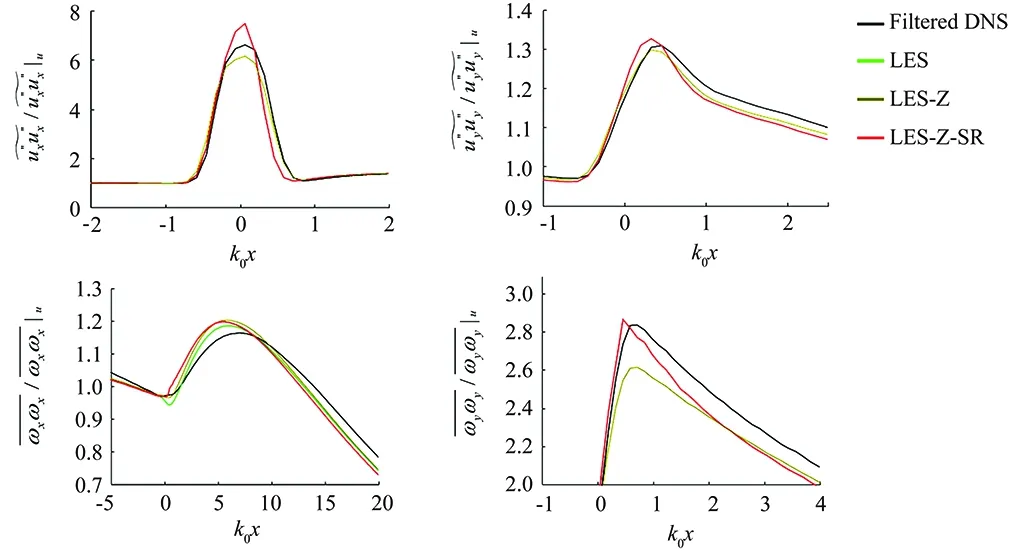
Fig.18 LES, WENO7fi, SR vs. no SR using LES-Z, zoom in the vicinity of the shock: Comparison to filtered DNS data of the statistics obtained by LES with different filtering procedures (with and without SR) on grid 389×642, M=1.5. Top row: streamwise (left) and transverse (right) Reynolds stress components Bottom row: streamuise (left) and transverse (right) vorticity components.

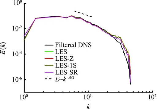
Fig.19 LES, WENO7fi, M=1.5, velocity spectrum: Comparison of velocity spectrum among different LES SGS filtering procedures (original SGS LES, LES-Z, LES-1S and LES-SR) at plane x=0 and the filtered DNS on grid 389×642.

2.3.2 Comparison of Two Different Filter DNS Operators

As the filter width is used for comparison with DNS data, one should consider the accuracy of such comparison.Therefore filtered DNS data may be considered as a reference solution only within the accuracy of filter width. The differences in filtered DNS data when using two different filter operators:

·The 5-point top-hat filter with coefficients (1/8, 1/4, 1/4, 1/4, 1/8) and width Δ≈4.2haccording to the estimate (15),

·The 7-point trapezoidal filter with coefficients (1/22, 1/11, 2/11, 4/11,2/11,1/11,1/22) and width Δ≈4.8h.

is reported in [45]. The top-hat filter has been used to obtain DNS filtered data plotted on previous figures. For more precise comparison of LES filtering modifieations, explicit LES will be considered in the future.

3 Concluding Remarks

The DNS results obtained by high order nonlinear filter schemes demonstrate a good agreement with the reference solution from Larsson & Lele [24]. The LES study confirms the results found by previous authors that the dynamic Germano LES model with a standard filtering procedure may loose accuracy due to a strong shock. The results obtained with the four modifications of the LES filtering procedure (LES-Z, LES-1S, LES-Z-SR and LES-1S-SR) using WENO7fi which are designed for improving the accuracy of the standard method have been presented. For the considered 3D shock-turbulence interaction problem all of these four modifications yield improvement in accuracy over the original dynamic SGS model. Our low dissipative WENO7fi is far more accurate than WENO7 using the same grid and models. It is noted that the turbulent Mach numberMt=0.16 for the test case considered here is quite low, and the SGS dissipation may be not high enough in comparison with numerical dissipation of the shock-capturing scheme. Different behavior of considered procedures is expected for high turbulent Mach numbers. These results are forthcoming. The SR procedure only increases the accuracy in certain flow variables over the no SR case. As originally expected, LES using the SR procedure helps improve the accuracy in the vicinity of the shock. A careful examination at the finer DNS grids presented earlier shows that the 4 peak values by SR indicate improved the accuracy over the no SR case. The simplified SR procedures might be a contributing factor to the lack of bigger accuracy improvement over the no SR procedure. It appears that the proposed LES using the SR model needs further refined consideration.

Acknowledgments:The support of the DOE/SciDAC SAP grant DE-AI02-06ER25796 is acknowledged. The authors are grateful to J. Larsson for providing the turbulent inflow and selected input data. The work has been performed with the first author as a postdoctoral fellow at the Center for Turbulence Research, Stanford University. Financial support from the NASA Aerosciences/RCA program for the second author is gratefully acknowledged.Work by the fifth author was performed under the auspices of the U.S. Department of Energy at Lawrence Livermore National Laboratory under Contract DE-AC52-07NA27344.

[1]Germano M, Piomelli U, Moin P, et al. A dynamic subgrid-scale eddy viscosity model[J].Physics of Fluids, 1991, 3(7): 1760-1765.

[2]Sagaut P, Germano M. On the filtering paradigm for LES of flows with discontinuities[J]. J. of Turbulence, 2005, 6(23):1-9.

[3]Grube N E,Martin M P. Assessment of subgrid-scale models and shock-confining filters in large-eddy simulation of highly compressible isotropic turbulence[C]//Orlando, Florida: 47th AIAA Aerospace Sciences Meeting Including The New Horizons Forum and Aerospace Exposition, 2009.

[4]Adams N A，Stolz S. A subgrid-scale deconvolution approach for shock capturing[J]. J. Comp. Phys.,2002, 178: 391-426.

[5]Yee H C,Sjögreen B. High order filter methods for wide range of compressible flow speeds[C]//Proc. of ICOSAHOM 09, Trondheim, Norway, 2009.

[6]Yee H C,Sjögreen B. Development of low dissipative high order filter schemes for multiscale Navier-Stokes/MHD systems[J]. J. Comput. Phys., 2007, 225:910-934.

[7]Sjögreen B,Yee H C. Multiresolution wavelet based adaptive numerical dissipation control for shock-turbulence computation[J]. J. Sci. Comput., 2004, 20:211-255.

[8]Yee H C, Sandham N D, Djomehri M J. Low dissipative high order shock-capturing methods using characteristic-based filters[J]. J. Comput. Phys.,1999, 150:199-238.

[9]Yee H C, Sjögreen B, Hadjadj A. Comparative study of three high order schemes for LES of temporally evolving mixing layers[J]. Commun. Comput. Phys., 2012, 12:1603-1622.

[10]Kotov D, Yee H C, Sjögreen B. Performance of improved high-order filter schemes for turbulent flows with shocks[C]//Proceedings of the ASTRONUM-2013, Biarritz, France, 2013.

[11]Kotov D, Yee H C, Hadjadj A, et al. High order numerical methods for LES of turbulent flows with shocks[C]//Proceedings of ICCFD8, Chengdu, Sichuan, China; also expanded version submitted to CiCP, July 14-18 2014.

[12]Lombardini M, Hill D J, Pullin D I. Atwood ratio dependence of Richtmyer-Meshkov flows under reshock conditions using large-eddy simulations[J]. J. Fluid Mech., 2011, 670:439-480.

[13]Johnsen E, Larsson J, Bhagatwala A V, et al. Assessment of high-resolution methods for numerical simulations of compressible turbulence with shock waves[J]. J. Comput. Phys., 2010, 229:1213-1237.

[14]Touber E,Sandham N. Comparison of three Large-Eddy Simulations of shock-induced turbulent separation bubbles[J]. Shock Waves, 2011, 19(6):469-478.

[15]Lo S -C, Blaisdell G A, Lyrintzis A S. High-order shock capturing schemes for turbulence calculations[J].J. for Num. Meth. in Fluids, 2010, 62(5):473-498.

[16]Ducros F, Ferrand V, Nicoud F, et al. Large-eddy simulation of the shock/turbulence interaction[J]. J. Comput. Phys., 1999, 152: 517-549.

[17]Kotov D V, Yee H C, Wray A, et al. Numerical dissipation control in high order shock capturing schemes for LES of low speed flows[C]//Proceedings of the ICOSAHOM 2014, Salt Lake City,Utah, 2014.

[18] Kotov D V, Yee H C, Sjögreen B. Performance of improved high-order filter schemes for turbulent flows with shocks[R]. Stanford: Center for Turbulence Research, Annual Research Briefs, 2013, 291-302.

[19]Yee H C, Sjögreen B, Hadjadj A. Comparative study of high order schemes for LES of temporal-evolving mixing layers[C]//Proc. of ASTRONUM-2010, San Diego, Calif. 2009.

[20]Kotov D, Yee H C, Hadjadj A, et al. High-order numerical methods for LES of turbulent flows with shocks[R]. Stanford: Center for Turbulence Research,Annual Research Briefs, 2014: 89-98.

[21]Wang W, Shu C -W, Yee H C, et al. High order finite difference methods with subcell resolution for advection equations with stiff source terms[J]. J. Comput. Phys., 2012, 231:190-214.

[22]Yee H C, Kotov D V, Wang W, et al. Spurious behavior of shock-capturing methods:Problems containing stiff source terms and discontinuities[C]//Proceedings of the ICCFD7, The Big Island, Hawaii, 2012,241:266-291.

[23]Harten A. ENO schemes with subcell resolution[J]. J. Comp. Phys., 1989, 83:148-184.

[24]Larsson J, Lele S K. Direct numerical simulation of canonical shock/turbulence interaction[J]. Physics of Fluids, 2009, 21(126101).

[25]Lilly D K. A proposed modification of the Germano subgrid-scale closure method[J]. Physics of Fluids, 1992, 4(3):633-635.

[26]Erlebacher G, Hussaini M Y, Speziale C G, et al. Toward the large eddy simulation of compressible turbulent flows[J]. J. Fluid Mech., 1992, 238:155.

[27]Lund T S. On the use of discrete fiters for large eddy simulation[R]. Stanford: Center for Turbulence Research, Annual Research Briefs. 1997: 83-95.

[28]Olsson P, Oliger J. Energy and maximum norm estimates for nonlinear conservation laws[R]. Technical Report 94.01, RIACS, 1994.

[29]Yee H C, Vinokur M, Djomehri M J. Entropy splitting and numerical dissipation[J]. J. Comput. Phys., 2000. 162: 33-81.

[30]Yee H C, Sjögreen B. Designing adaptive low dissipative high

order schemes for long-time integrations[M]//Drikakis D, Geurts B. Turbulent Flow Computation. Kluwer Academic, 2002.

[31]Ducros F, Laporte F, Soulères T, et al. High-order fluxes for conservative skew-symmetric-like schemes in structured meshes: Application to compressible flows[J]. J.Comp. Phys., 2000, 161: 114-139.

[32]Sjögreen B,Yee H C. On skew-symmetric splitting and entropy conservation schemes for the Euler equations[C]// Proc. of the 8th Euro. Conf. on Numerical Mathematics & Advanced Applications(ENUMATH 2009). Uppsala, Sweden: Uppsala University, 2009.

[33]Olsson P. Summation by parts, projections, and stability I[J]. Math. Comp., 1995, 64:1035-1065.

[34]Sjögreen B,Yee H C. On tenth-order central spatial schemes[C]//Proceedings of the Turbulence and Shear Flow Phenomena 5 (TSFP-5).Munich, Germany: 2007.

[35]Vinokur M,Yee H C. Extension of efficient low dissipative high-order schemes for 3-d curvilinear moving grids[J]// Frontiers of Computational Fluid dynamics, World Scientific, 2002: 129-164.

[36]Ciment M,Leventhal S H. Higher order compact implicit schemes for the wave equation[J]. Math. Comp.,1975, 29: 985-994.

[37]Sandham N D, Li Q, Yee H C. Entropy splitting for high-order numerical simulation of compressible turbulence[J]. J. Comp. Phys., 2002,178:307-322.

[38]Yee H C,Sjögreen B. Simulation of Richtmyer-Meshkov instability by sixth-order filter methods[J].Shock Waves, 2007, 17:185-193.

[39]Hadjadj A, Yee H C, Sjögreen B. LES of temporally evolving mixing layers by an eighth-order filter scheme[J]. Int. J. for Num. Meth. in Fluids, 2012, 70:1405-1427.

[40]Hadjadj A, Dubos S. Large eddy simulation of supersonic boundary layer at M = 2.4[C]//Braza M,Hourigan K.Proceeding of the IUTAM Symposium on Unsteady Separated Flows and their Control. Springer, 2009. e-ISBN 978-1-4020-9898-7.

[41]Bermejo-Moreno I, Larsson J, Lele S K. LES of canonical shock-turbulence interaction[R].Stanford: Center for Turbulence Research, Annual Research Briefs, 2010: 209-222.

[42]Shu C-W, Osher S. Efficient implementation of essentially non-oscillatory shock-capturing scheme, II[J]. J. Comp. Phys., 1989, 83:32-78.

[43]Lee S, Lele S K, Moin P. Interaction of isotropic turbulence with shock waves: Effect of shock strength[J]. J. Fluid Mech., 1997, 340:225-247.

[44]Ristorcelli J R, Blaisdell G A. Consistent initial conditions for the DNS of compressible turbulence[J].Physics of Fluids, 1997, 9(4).

[45]Kotov D, Yee H C, Hadjadj A, et al. High order numerical methods for the dynamic SGS model of turbulent flows with shocks[J]. Commun. Comput. Phys., 2016, 19: 89-98.

0258-1825(2016)02-0190-14

含激波的湍流流动高精度大涡数值模拟方法

D.V. Kotov1, H. C. Yee2,*, A. Wray2, A. Hadjadj3, B. Sjögreen4

(1. Center for Turbulence Research, Stanford University, Stanford, CA 94305, USA; 2. NASA Ames Research Center, Moffett Field, CA, 94035, USA; 3. CORIA UMR 6614 & INSA de Rouen, 76800 St-Etienne du Rouvray, France; 4. Lawrence Livermore National Laboratory, Box 808, L-422, Livermore, CA 94551, USA)

针对采用亚格子模型进行含激波的湍流流动模拟时会面临激波附近的精度损失问题，考虑从通过亚格子模型以及数值模拟方法两方面的改进来实现湍流流动大涡模拟的精度提高。大涡模拟采用了Yee及Sjögreen(2009)提出的高阶低耗散方法。该方法采用自适应的流场探测器以控制计算中所需区域的数值耗散，并考虑对动力学模型采用在激波位置使用Sagaut 和Germano(2005)提出的单边亚格子过滤器和(或)直接禁用亚格子项等方法加以改进。对于标准的马赫数1.5和3条件下的激波-湍流干扰问题，上述新方法相较于全区域采用亚格子模型的方法均表现出了相似的精度提升。同时实现的数值精度改进方案采用了Harten的亚单元分辨过程来定位和锐化激波，并在精确激波位置附近的网格点处采用了单边测试滤波。

高阶低耗散格式; Germao模型; 大涡模拟滤波; 直接数值模拟方法; 亚单元分辨格式; 激波-湍流干扰

V211.3

A doi: 10.7638/kqdlxxb-2016.0009

*helen.m.yee@nasa.gov

format: Kotov D V, Yee H C, Wray A, et al. High order numerical methods for LES of turbulent flows with shocks[J]. Acta Aerodynamica Sinica, 2016, 34(2): 190-203.

10.7638/kqdlxxb-2016.0009. Kotov D V, Yee H C, Wray A, 等. 含激波的湍流流动高精度大涡数值模拟方法(英文)[J]. 空气动力学学报, 2016, 34(2): 190-203.

Received date： 2016-02-04; Revised date：2016-03-25