Numerical analysis of the unsteady behavior of cloud cavitation around a hydrofoil based on an improved filter-based model*
2015-11-25ZHANGDesheng张德胜WANGHaiyu王海宇SHIWeidong施卫东
ZHANG De-sheng (张德胜), WANG Hai-yu (王海宇), SHI Wei-dong (施卫东),
ZHANG Guang-jian (张光建)1, Van ESCH B. P. M. (Bart)2
1. Research Center of Fluid Machinery Engineering and Technology, Jiangsu University, Zhenjiang 212013,China, E-mail:zds@ujs.edu.cn
2. Department of Mechanical Engineering, Eindhoven University of Technology, Eindhoven 5600MB, The Netherlands
Numerical analysis of the unsteady behavior of cloud cavitation around a hydrofoil based on an improved filter-based model*
ZHANG De-sheng (张德胜)1, WANG Hai-yu (王海宇)1, SHI Wei-dong (施卫东)1,
ZHANG Guang-jian (张光建)1, Van ESCH B. P. M. (Bart)2
1. Research Center of Fluid Machinery Engineering and Technology, Jiangsu University, Zhenjiang 212013,China, E-mail:zds@ujs.edu.cn
2. Department of Mechanical Engineering, Eindhoven University of Technology, Eindhoven 5600MB, The Netherlands
2015,27(5):795-808
The unsteady cavitation evolution around the Clark-Y hydrofoil is investigated in this paper, by using an improved filter-base model (FBM) with the density correction method (DCM). To improve the prediction accuracy, the filter scale is adjusted based on the grid size. The numerical results show that a small filter scale is crucial for the unsteady simulations of the cavity shedding flow. The hybrid method that combines the FBM and the DCM could help to limit the overprediction of the turbulent viscosity in the cavitation region on the wall of the hydrofoil and in the wake. The large value of the maximum density ratio ρl/ρv,clippromotes the mass transfer rate between the liquid phase and the vapor phase, which results in a large sheet cavity length and the vapor fraction rise inside the cavity. The cavity patterns predicted by the improved method are verified by the experimental visualizations. The time-average lift, the drag coefficient and the primary oscillating frequencyStfor the cavitation number σ=0.8, the angle of attack,α=8o, at a Reynolds number Re=7×10⁵are 0.735, 0.115 and 0.183, respectively, and the predicted errors are 3.29%, 3.36% and 8.93%. The typical three stages in one revolution are well-captured, including the initiation of the sheet/attached cavity, the growth toward the trailing edge (TE) with the development of the re-entrant jet flow, and the large scale cloud cavity shedding. It is observed that the cloud cavity shedding flow induces the vortex pairs of the TE vortices in the wake and the shedding vortices. The positive vorticity vortex of the re-entrant jet and the TE vortices interacts and merges with the negative vorticity vortex of the leading edge (LE) cavity to produce the shedding flow.
filter-based model (FBM), density correction method, cloud cavitation, hydrofoil, unsteady behavior
Introduction
Cavitation occurs when the pressure is decreased below the vaporization pressure of the liquid. Cavitation often leads to erosion damage, noise, vibration and hydraulic performance deterioration due to its highly unstable behavior[1,2]. In order to control the damage induced by cavitation on hydraulic machinery, it is very important to study the mechanism of the unsteady cloud cavitation.
To improve the understanding of the complex cavitating flows, many experimental and numerical investigations were conducted for the cloud cavitation,especially, for the hydrofoils. Wang et al.[3]and Matsunari et al.[4]investigated the hydrofoil Clark-Y in different stages of the cavitation flow field using the high speed photography and the laser doppler anemometer, and also observed the U-shaped cavity structure. Leroux et al.[5,6]studied the local instability and the characteristics of the cloud cavitation by employing the pressure sensors along the suction side of the hydrofoil, and measured the lift and drag coefficients and captured pictures at the transient instants. It is widely believed that the cavity instability originates from a process involving the growth of the re-entrant jet,the cavity cloud shedding, and a shock wave phenomenon due to the collapse of a large cloud cavitation. Callenaere et al.[7]experimentally investigated the instability of a partial cavity induced by the development of a re-entrant jet on a diverging step. The results suggest that the adverse pressure gradient and the cavity thickness are critical to the re-entrant jet instability.
It is well known that the cavitation model and the turbulence model are essential parts in simulating the cavitating flows. The homogeneous cavitation models based on the Reyleigh-Plesset equation including the Singhal model, the Zwart-Gerber-Belamri model and the Schnerr and Sauer model, are mostly used and validated by modeling the cavitating flows in hydrofoils,propellers and pumps[8,9]. Recently, in the cavitation simulation, the turbulent viscosity overestimation for the cavitating flows by using the Reynolds averaged Navier-Stokes (RANS) method has attracted much attention, and it was confirmed by many studies[8,9]based on the original RANS turbulence models. To improve the prediction accuracy, the large eddy simulation (LES), the direct numerical simulation (DNS),and the lattice Boltzmann method (LBM) might be used to model the unsteady cloud cavitation and they can offer convincing time-dependent results. However,the high demand for the grid density, especially, in the boundary layer and the computational cost make them unpractical in most industrial applications.
In recent years, hybrid models provide a solution for the overpredition of turbulent viscosity in the cavitating flow. The partial averaged Navier-Stokes(PANS)[10,11]is a hybrid of the DNS and the RANS, in which the key is to determine the ratio of the unresolved-to-total kinetic energy,fk, and the ratio of the unresolved-to-total dissipation,fe[12]. Johansen et al.[13]proposed a filter-based model (FBM) combining both the standard k-εand one equation LES[14]by introducing a filter scale. Unlike the LES and DES,the filter in the FBM is not related with the grid scale,which makes the grid independent simulations possible. In addition, another way to tackle the deficiency in predicting the cavitating flows is the density correction method (DCM) proposed by Reboud[9]and implemented[6,8]in the classic RANS models. This method can limit the turbulent viscosity in the vapor-liquid mixture region effectively.
Based on these ideas, with consideration of the advantages of both the FBM and the DCM, this paper proposes an improved FBM, coupled with the DCM and the suitable maximum density ratio. The improved turbulence model is validated by the cloud cavitation shedding flow around the Clark-Y hydrofoil as compared with the experimental results. The Zwart-Gerber-Belamri cavitation model is employed to compute the mass transfer between the vapor and the water. The effect of the maximum density ratio is analyzed to increase the prediction accuracy as well.
1. Numerical method and setup
1.1 Governing equations
In the vapor/liquid two-phase mixture model[15],the fluid is assumed to be homogeneous, so the multiphase fluid components are assumed to share the same velocity and pressure. The continuity and momentum equations for the mixture flow are as follows:
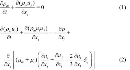
where ρmis the density of the mixture,uiis the instant velocity in the directioni,p is the mixture pressure,µmis the mixture laminar viscosity and µtis the turbulent viscosity, which is obtained by the following turbulence model.
The mixture density ρm, is defined as

whereρandαare the density and the volume fraction, respectively. The subscriptsvandl refer to the vapor and liquid components, respectively.
1.2 Filter-based density corrected model
The original two-equation models may over-predict the turbulent viscosity in the cavitation region, result in an over-prediction of the turbulent viscosity,and make the re-entrant jet to lose momentum and thus make the jet unable to cut across the cavity sheet. To improve the simulations by taking into account the influence of the local compressibility effect on the turbulent closure model, the DCM based on the local mixture density was proposed by Reboud[16], and then Coutier-Delgosha et al.[9]and Dular et al.[17]showed that DCM could help to reduce the turbulent viscosity in the RNG k-εturbulence model.

In this paper, the FBM[13,18]is used based on the original RNG k-εturbulence model. A filter-based density corrected model that combines the advantages of both the FBM and DCM models is proposed. A hybrid model for the filter functionF and the DCM is added in the turbulent viscosity equation to reduce the turbulent viscosity and limit the overprediction of the turbulent eddy viscosity in the ca[1v3i,1t8a]ting regions on the hydrofoil wall and in the wake.
1.3 Cavitation model
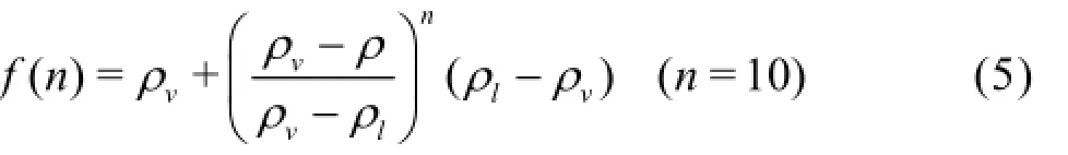
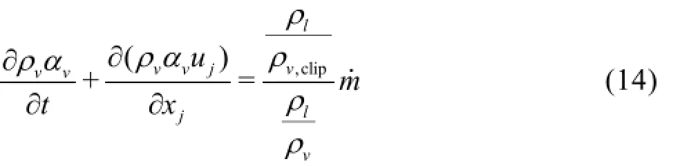
The cavitation model describes the mass transfer between the liquid and the vapor. In the present paper,the Zwart-Gerber-Belamri cavitation model is used,which is derived from a simplified Rayleigh-Plesset equation with neglect of the second-order derivatives of the bubble radius[15]. The vapor density is clipped in a user-controlled fashion by the maximum density ratio ρl/ρv,clipto control the numerical stability and accuracy. The maximum density ratio is used to clip the vapor density for all terms except the cavitation source term itself, which is the true density specified as the material property.

The vapor volume fraction is governed by the following equations: wherem˙is the cavitation source term, which controls the mass transfer rates between the liquid and the vapor.ρl,ρvand ρv,clipare the liquid density, the vapor density, and the clipped vapor density calculated according to the maximum density ratio.pvis the saturated liquid pressure,p is the local fluid pressure.Feand Fcare empirical coefficients for the vaporization and the condensation process.αnucis the non-condensable vapor fraction, and RBis the bubble size. These empirical constants are set as Fe=50,based on the work of Zwart et al.[15], which were also validated in various studies[19].
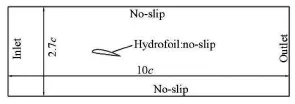
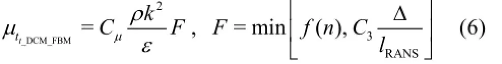
Fig.1 Computational domain and boundary conditions
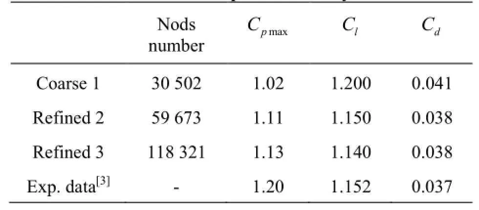
Table 1 Results of mesh independence study
1.4 Computational domain, meshing and boundary conditions
The experiment of the 2-D Clark-Y hydrofoil with chord length c =0.07m, angle of attack α=8o, was conducted by Wang et al.[3]The computational domain is shown in Fig.1, which is installed at the same location in the water channel. The leading edge is set as the origin of the coordinates. The distance between the upper wall and the bottom wall is2.7c(chord length), the outlet is10c away from the inlet and the leading edge of the hydrofoil is3c from the inlet.

Fig.2 The structural mesh around the hydrofoil
The medium is water and water vapor at 25oC. The main boundary conditions are as follows: the inlet velocity Uin=10m/s, the corresponding Reynolds numberRe=7×10⁵, the low inlet turbulence intensity (1%), and the pressure outlet. No-slip wall is adopted in the upper and bottom walls. The simulations are conducted by using the CFD code ANSYS CFX. The pressure-velocity direct coupling method is used to solve the governing equations. The high resolution scheme is used for the convection terms with the central difference scheme used for the diffusion terms in the governing equations. The unsteady second-order implicit time integration scheme is used for the transient term. The unsteady cavitating flow simulations start from a steady non-cavitation flow results. The time step∆t=0.1msis used for the revolution calculation. During the unsteady calculation, the convergence in each physical time step is achieved through 4 to 10 iterations when the root mean square (RMS) residual is dropped below 10-5.
The structural grid is established in the computational domain. A C-type block is used around the hydrofoil, considering the round shape in the head of the hydrofoil and the sharp trailing edge. The lift coefficient and the drag coefficient are defined as:
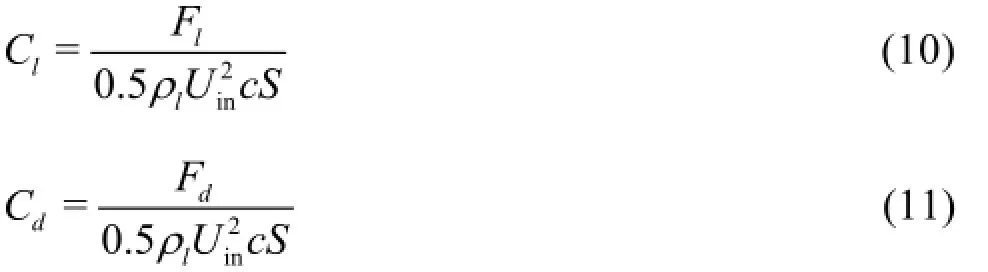
where Fland Fdare the lift force and the drag force on the hydrofoil, respectively,Sis the span of the hydrofoil.
The mesh independence study is shown in Table 1. The results of the refined grid 2 with a medium density grid are nearly the same as those of the refined grid 3, and they agree well with the experimental results. Thus, the refined grid 2 is used in this paper. Figure 2 presents the overall mesh around the Clark-Y hydrofoil and the local meshes near the leading edge(LE) and the trailing edge (TE). The y+value on the surface of the hydrofoil varies between 20-75 with an average of 31, which satisfies the demand of the standard wall function, and makes sure that the first node is located higher than the logarithmic layer.
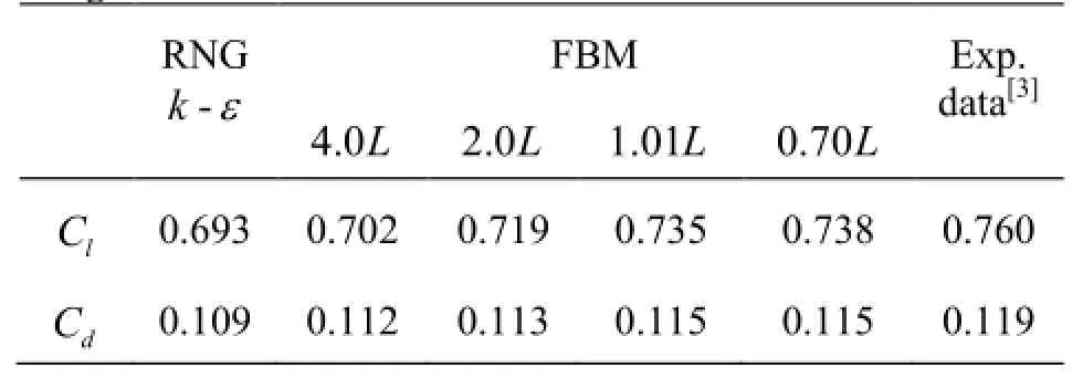
Table 2 Time-average lift and drag coefficients predicted using different filter sizes
1.5 Effect of filter scale in FBM
The FBM combines the advantages of the RANS and the LES, but it requires a reasonable filter scale∆. It is indicated in Eq.(6) that when the filter scale∆is too large, the FBM is degenerated into the RANS, which makes the filter meaningless. When the filter scale∆is very small, the FBM is almost the one-equation LES model, and the demand on the grid number and the computational resource is increased. In order to obtain a proper filter scale∆, we make tests of0.7L,1.01L,2.0L,4.0L in the FBM and the RNG k-εin the unsteady cavitation simulation around the Clark-Y hydrofoil with a cavitation numberσ=0.8. The time-averaged lift and drag coefficients in 5 cycles are presented in Table 2. Both the lift and drag coefficients predicted by1.01Land 0.7Lapproach the experimental results. When the filter scale is reduced to0.7L, the predicted results tend to be stable.
Thus, a proper filter scale is critical to the prediction accuracy of the simulation. To some extent, asmaller filter size can increase the FBM capacity to resolve vortexes in finer scales. However, the filter size is also limited by the grid scale. In the present simulations, the filter scale ∆=1.01Lis used finally according to the grid size.

Fig.3 Comparison of cavity evolution computed using different turbulence models
2. Results and discussions
2.1 Density correction method based on FBM
In order to validate the improvement on the FBM,the two turbulence models mentioned above are used in the unsteady calculation of the cloud cavitation around the hydrofoil, with a cavitation number σ= 0.8. The predicted results are illustrated in Fig.3. As the LES equation is used to resolve the fully developed turbulence near the wall of the hydrofoil and in the wake, the cavity cloud shedding is observed in both simulations. A significant difference is found of the predictions of the vapor fraction inside the cavity and the length of the sheet cavity.
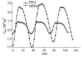
Fig.4 Comparison of vapor volume in the whole computation domain calculated by different models
To validate the effect of the DCM, the cavity volumes in the whole flow field calculated by different turbulence models are calculated as shown in Fig.3, in which the cavity volume Vcavis defined as
wheren is the number of the grid elements,αiis the vapor volume fraction of every element,Viis the volume of each element. Three cycles of the cavity volume variation are shown in Fig.4. The time-averaged cavity volume obtained by the MFBM is about 3 times as that obtained by the FBM, as is evident in the discrepancy presented in Fig.3.
Figure 5 shows the turbulent viscosity distribution calculated by different turbulence models. The original RNGk-εmodel overpredicts the turbulent viscosity in the cavity regions, which would hinder the sheet cavity fracture and the cloud cavity shedding. As mentioned in Section 1.2, the FBM model can solve the overprediction problem of the turbulent viscosity,especially in regions with large turbulence scales. Based on Eq.(6) of the FBM, the flow field with a large turbulence scale is simulated by using the LES single-equation, which predicts a more reasonable turbulent viscosity. However, the FBM model still has some limitations, e.g., in the small-scale turbulent region and the near-wall region, it turns into the RNG k-εmodel, which means that the traditional twoequation turbulence model is used for the simulation without taking into account the compressible effects of the vapor-liquid region. To solve this problem, the DCM is applied in the FBM. The FBM combined with the DCM could predict a reasonable distribution of the turbulent viscosity as shown in Fig.5(c). The predicted unsteady features of the cloud cavitation also agree well with the experimental visualizations in the following simulations.
2.2 Effect of maximum density ratio
In order to ensure that the simulation is stable,the maximum density ratioρl/ρv,clipis introduced tocontrol the vapor density. The vapor volume fraction is controlled by
where ρv,clipis calculated based on the maximum density ratioρl/ρv,clip. Note that the genuine physical gas density is used in the cavitation source termm.
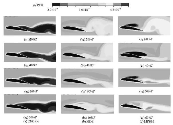
Fig.5 Distributions of turbulent viscosity calculated by different turbulence models,Re=7×10⁵,α=8o,σ=0.8
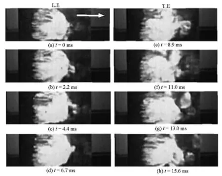
Fig.6 Experimental sheet cavity patterns (Re=7×10⁵,α=8o,σ=1.4). The arrow indicates main flow direction

Fig.7 Predicted cavity patterns and local velocity vector distributions with different ρ/ρ.Re=7×105,α=8o,σ=1.4lv,clip
ρv,clip=ρl/ρv/ρl/ρv,clipρvis substituted into Eq.(11). So Eq.(11) can be written as
Equation (12) shows that the cavitation mass transfer rate (the right term) is strongly related with the maximum density ratio. It was suggested in the previous studies[12]thatalso affects the compressibility in the gas-liquid mixture region and the gas-liquid transfer rate.
Figure 6 presents the experimental visualizations[3]on the Clark-Y hydrofoil with the cavitation number σ=1.4,α=8o. The sheet cavity is attached on the suction side of the hydrofoil from the leading edge to0.4c. The body of the cavity is stable, but the rear region of the sheet is unstable, with a 3-D nature,and rolls up into a series of bubbly eddies that shed intermittently.
In order to investigate the influence of the maximum density ratio, three values are tested in this paper. They are 1 000 (the default setting in the CFX),20 000 and 43 197 (the actual vapor-liquid density ratio). In view of the fact that the sheet cavity is quasi stable, the RNGk-εis employed here for the unsteady simulation. The numerical results are presented in Fig.7. A steady attached sheet cavity is obtained with the default maximum density ratio 1 000, but the unstable circulation flow in region A is not observed. The numerical results predicted by the maximum density ratio 20 000 and 43 197 include a quasi-unsteady sheet cavity, with a clockwise vortex induced by the interaction of the re-entrant jet and the main flow at the closure of the cavity as shown in region A. Disturbed by the vortex, small bubble clusters shed from the rear part of the cavity, which is consistent with the experiment. So, a largeρl/ρv,cliphelps to increase the mass transfer rate between the liquid phase and the vapor phase, improving the vapor volume fraction of the cavity body. With the increase of ρl/ρv,clip, the cavity length increases accordingly. The cavity length is0.24cwhenρl/ρv,clip=1000, and is far from the experiment observation of0.4c. It agrees with the result in literature[20], which indicates that the default setting value of ρl/ρv,clipin the ANSYS CFX underestimates the cavitation development. In addition, the cavity length is approximately0.42cfor the maximum density ratio of 20 000 or 43 197, which is almost the same as the experimental result. In Table 3, the predicted lift coefficients, the drag coefficients, the cavity area, the cavity length are compared with experiment results.
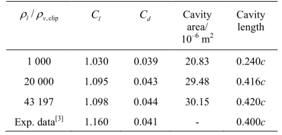
Table 3 Influence of different maximum density ratios on the results of cavitation simulation
In general, when the maximum density ratio is equal to 20 000 or 43 197, the results are quite close. However, it is confirmed that the results predicted by the default value of 1 000 show a significant prediction error compared with the experimental data. In summary, the maximum density ratio has a major influence on the cavitation calculation. Although the default value 1 000 is beneficial for the convergence and the numerical stability, in this paper, the maximum density ratio ρl/ρv,clip=20000is used in the following simulations.
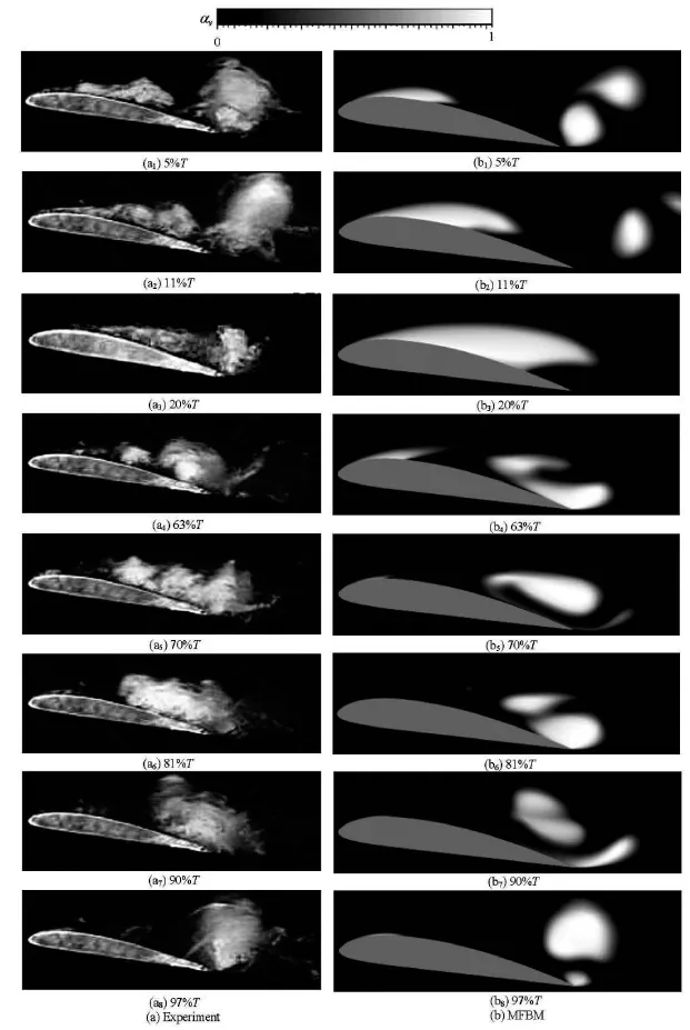
Fig.8 Comparison of cavitation evolution in one typical cycle,Re=7×10⁵,α=8o,σ=0.8
2.3 One cycle of cloud cavitation
A comparison of the cloud cavitation evolution obtained by experiment and simulation in one typical period is presented in Fig.8, in which the experimental results are provided by Wang[4].
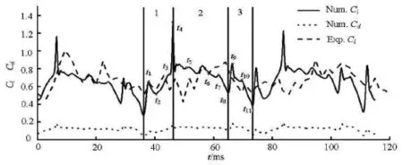
Fig.9 Time evolution of lift and drag coefficients in cloud cavitation
It is observed that the predicted cloud cavitation assumes a distinct quasi-periodic pattern, the cavity visualizations are made through the side view according to 5%, 11%, 20%, 63%, 70%, 81%, 90% and 97% of each corresponding cycle. The period timeT of the cloud cavitation is estimated as 38.3 ms, which is shorter than the experimental time T=40ms. The predicted patterns of every stage during the unsteady cloud cavitation compare well with the experimental visualizations, including the initiation of the attached cavity, the growth toward the TE, and the subsequent cloud shedding. As shown in Fig.8, first of all, the attached sheet cavity is expanded up to the TE of the hydrofoil at5%Tand at20%T, followed by the breakup near the LE due to the re-entrant jet at63%T through 90%T, and then a complete convection of the cloud cavity into the wake is observed at97%T.
2.4 Unsteady behavior of cloud cavitation
The growth, the unsteady shedding and the collapse of the cavity significantly influence the pressure distribution on the suction side of the hydrofoil. Consequently, the lift coefficients show a quasi-periodic characteristics corresponding to the unsteady cavity pattern. Three time-dependent revolutions of the lift and drag coefficients obtained by experiment and simulation are presented in Fig.9.
The predicted lift coefficient compares well with the experimental data. However, the numerical results fluctuate in a much larger extent. The lift coefficient shows remarkable peaks and valleys, corresponding to the collapse and the shedding of the bubble cloud. The notable unsteady pressure fluctuation induces the rapid changes of the lift coefficient. The experimental results might be limited by the response frequency of the pressure sensor. The lift coefficient shares the same trend with the drag coefficient, suggesting a strong correlation with the cavity shedding flow. The time average predicted lift coefficient in the present calculation isCl=0.735, which is 3.30% lower than the experimentally measured values of 0.760 and 0.119, and are more accurate than the RANS results.

Fig.10 Frequency spectrum of lift coefficient in cloud cavitation
The predicted time-dependent lift coefficient is processed by using the Fast Fourier Transformation,so the spectrum of the lift coefficient is obtained as shown in Fig.10. The main frequency is normalized by the chord length c and the upstream velocity Uin,St=fc/Uin. So the predicted primary oscillating frequency St1=0.183compares well with the experimental valueSt1=0.167. The primary frequency of the hydrodynamic fluctuations is induced by the unsteadiness of the cavity, and is in agreement with the cloud cavity shedding frequency, as is verified in the present simulations. The predicted second oscillating frequencySt2=0.365is also quite near the experimental data St2=0.340. Besides, there exist frequencies with high power density when the Strouhal numberSt ranges from 0.4 to 1.0. These frequencies may come from the instability of the vortex structures, which are interacted with the unsteady cavitating shedding flow.
The variable lift coefficient has a close relation with the evolution of the cloud cavitation. One typical cloud cavitation period could be divided into 3 stages.According to the cavity patterns, the detailed analysis is presented as follows.
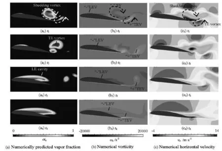
Fig.11 Distributions of cavity pattern, vorticity and horizontal velocity at stage 1
2.4.1 Initiation and growth of the attached cavity
The first stage includes the initiation of the sheet attached cavity, the growth to the TE and the collapse of the cloud cavity in the previous cycle, in which 4 typical instants from t1to t4are selected to see the cavity patterns, the vorticity and the horizontal velocity as shown in Fig.11. Here, the vorticityωzis defined as ness. The lift coefficient reaches a local maximum as shown in Fig.9, corresponding to the time when the LE sheet cavity grows to the maximum at t4, covering almost the whole suction side of the hydrofoil. This is due to the high pressure wave caused by the collapse of the main cloud cavity. It indicates that the cloud cavity collapse process has a more severe impact on the pressure coefficients than the TE vortex collapse. The shedding vortex and the TE vortex also can be identified by the horizontal velocity distribution, in which it has a negative velocity in the opposite direction of the main flow. The vortex of negative velocity is mainly located in the vortex pair shedding region in the previous cycle. Thus, when the cloud cavity moves downwards and collapses, the size of the reversed flow region is decreased.
2.4.2 The development of re-entrant jet flow
The second stage is characterized by the interaction between the re-entrant jet and the cavity vortices as well as the cavity interface. The four typical instants from t5to t8are illustrated in Fig.12. When the TE sheet cavity grows to the maximum size, the cavity interface becomes bubbly as shown in Fig.12(t5). At this time point, the adverse pressure gradient is strong enough to overcome the weak momentum of the

At t1, the low pressure at the head of the hydrofoil produces an attached sheet cavity. At the same time, a shedding vortex with a negative vorticity(“-”SV) and the counterclockwise TE vortex with a positive vorticity (“+”TEV) co-exit at the rear of the hydrofoil, while the leading edge vortex in the sheet cavity region has also a negative vorticity(“-”LEV). The lift coefficient drops att2because of the collapse of the TE vortex which induces a pressure decrease on the surface of the hydrofoil. Att3and t4, the attached sheet cavity continues to expand in length and thick-flow confined by the near-wall region, so the re-entrant jet forms and moves backwards from the TE to the LE as shown in the right column of Fig.12, in which the vortex with negative velocity near the wall indicates the re-entrant jet. Affected by the re-entrant jet, the vapor-liquid interface is extremely turbulent. With the migration of the re-entrant jet towards the leading edge, the sheet cavity is cut off into two main cavities at t6, which are the stable LE attached sheet cavity and the unstable detached cloud cavity vortex(“-”SV ) at the rear of the hydrofoil. Meanwhile, the TEV also develops. When the local pressure inside the TEV is lower than the saturated liquid pressure att7,the TEV cavity appears. In this stage, the re-entrant jet(REJ), the LEV and the TEV interact with each other, inducing the fluctuation of the lift coefficient. As shown in the middle column of Fig.12, the positive vorticity of the TE in the wake of the hydrofoil is incentive to the formation of the TEV cavity. The shedding vortex (“-”SV) with negative vorticity is driven by the interaction between the re-entrant jet (“+”REV)and the main flow as shown in Fig.13. The analysis mentioned above indicates that there is a counter-rotating vortex pair near the TE including a “-”SV and a“+”REV. As shown in the right column of Fig.12, the re-entrant jet moves backward to the LE along the surface of the suction side, and interacts with the LE sheet cavity.
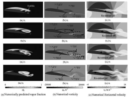
Fig.12 Distributions of cavity pattern, vorticity and horizontal velocity at stage 2
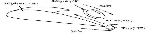
Fig.13 Vortex pairs induced by re-entrant jet and main flow
To understand the cut-off of the stable attached cavity, Fig.14 presents the distributions of the velocityvector and the pressure coefficient around the hydrofoil at t7. The re-entrant jet plays an important role to trigger the unsteady cavitation dynamics. The front location of the re-entrant jet, where the local high pressure contributes to the condensation of vapor. This is the key reason for the cut-off of the attached cavity. However, the intensities of the re-entrant jets, which can be identified by the maximum adverse velocities,-7.04 m/s, -6.4 m/s, -6.09 m/s and -5.71 m/s respectively, fromt5to t8in the second stage, decrease gradually because of the drop of the reverse pressure gradient. Att8, the re-entrant jet almost reaches the LE, resulting in the decrease of the lift coefficient. The shedding vortex (“-”SV ) and the LE vortex(“+”TEV) are entrained by the main flow, which also interact with the re-entrant jet (REJ). The vortex pair sheds slowly and convects downstream.
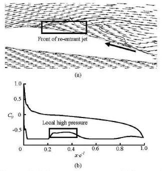
Fig.14 Distributions of velocity vector and pressure coefficient around hydrofoil at t7
The distributions of the time-averaged horizontal velocity uat three typical locations are shown in Fig.15, wherexis the distance to the LE andyis the distance to the surface of the hydrofoil. The numerically predicted velocity distributions compare well with the experimental results . Atx/c=0.4, the distribution of the time-averaged velocity shows a large velocity gradient in the near-wall region, but the reentrant jet does not appear at this position. Atx/c= 0.8, the time-averaged velocity near the wall is negative, indicating the appearance of the re-entrant jet. With the increase of the wall distance, the time averaged velocity approaches the main flow velocity. At x/c =1.2, theycomponent of the time-averaged horizontal velocity varies greatly. It suggests that the wake of “+”TEV interacts with “-”SV and has a large velocity gradient near the TE of the hydrofoil, which is also induced by the re-entrant jet.
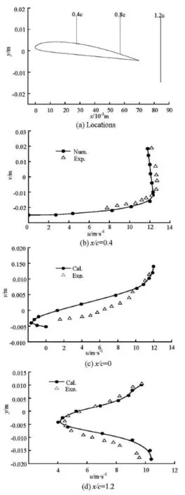
Fig.15 Time-averaged u -velocity at different locations

Fig.16 Distributions of cavity pattern, vorticity and horizontal velocity at stage 3
2.4.3 Large scale cloud cavity shedding
Stage 3 mainly consists of the formation and the convection of the cavity cloud. As shown in Fig.16,the LEV, the SC, the TEV and the REV interact with each other when the large cloud cavity mixture moves downward and sheds. The re-entrant jet reaches the LE of the hydrofoil at t9, eliminating the attached cavity. At this time point, the cavity at the rear of the hydrofoil leaves the surface and sheds downstream in a form of cloud cavity. The hydrofoil surface is free of cavity, which is the main reason why the lift coefficient can reach the local maximum. Fromt9to t11, the lift coefficient drops immediately due to the shedding of the cloud cavity. As shown in the horizontal velocity distribution in Fig.16, the decrease of the reverse pressure gradient fails to overcome the momentum of the main flow, in other words, the re-entrant jet starts to shrink to the TE. Att9and t10, the interaction between the SV and the TEV is observed, and followed by the completely convection of the cloud cavity into the wake. The development of the TEV expands the positive vorticity region, the interaction between the SV and the REJ contributes to the negative vorticity. The vorticity of the LEV enhances and the LE cavity appears again and begins to grow in the next cycle at t11.
In general, the strong correlation between the vorticity and the cavity shape is observed from the comparison of the contours of the vapor volume fraction and the vorticity in Figs.9-11. The re-entrant jet,which plays a significant role in the evolution of the cloud cavitation, induces the counter-rotating vortex pair including “-”SV and “+”TEV, which are merged into the large-scale cloud cavity. Finally, it sheds and collapses in the wake of the hydrofoil.
3. Conclusions
(1) An improved FBM model with the hybrid method combining the filter-based model with the density correction method is shown capable of limiting the turbulent viscosity in the cavitating flow. To improve the prediction accuracy, the effect of the filter scale∆is analyzed based on the grid scale, as well as the maximum density ratio ρl/ρv,clipin the Zwart-Gerber-Belamri cavitation model. The results show that the large value ofρl/ρv,clipcan increase the cavity length and the vapor fraction inside the cavity around the Clark-Y hydrofoil. The predicted unsteady features of the cloud cavitation in one cycle compare well with the experimental visualizations. The predicted time-averaged lift coefficient and drag coefficientas well as the Strouhal number are only 3.29%, 2.36% and 9.58%, respectively.
(2) The predicted lift and drag coefficients show a quasi-periodic variation, corresponding to three typical stages: (a) the initiation and growth of the attached cavity, (b) the development of the re-entrant flow, (c)the large-scale cloud cavity shedding. The unsteady cavity patterns in one cycle are well-captured to see the dynamics of the cloud cavitation.
(3) It is found that the shedding vortex TE with negative vorticity (“-”SV) and the counterclockwise TE vortex with positive vorticity (“+”TEV) co-exit at the rear of the hydrofoil during the cloud cavity shedding. This vortex pair is induced by the re-entrant jet and the main flow. The positive vorticity vortex of the re-entrant jet and the TE vortices interacts and merges with the negative vorticity vortex of the LE cavity to produce the shedding flow.
Acknowledgement
References
[1] BRENNEN C. E. Cavitation and bubble dynamics[M]. New York, USA: Cambridge University Press, 2013.
[2] BRENNEN C. E. Hydrodynamics of pumps[M]. New York, USA: Cambridge University Press, 2011.
[3] WANG G., SENOCAK I. and SHYY W. et al. Dynamics of attached turbulent cavitating flows[J]. Progress in Aerospace Sciences, 2001, 37(6): 551-581.
[4] MATSUNARI H. Experimental/numerical study on cavitating flow around clark Y 11.7% hydrofoil[C]. Proceedings of the 8th International Sympositm on Cavitation, (CAV 2012). Singapore, 2012.
[5] LEROUX J.-B., ASTOLFI J. A. and BILLARD J. Y. An experimental study of unsteady partial cavitation[J]. Journal of Fluids Engineering, 2004, 126(1): 94-101.
[6] LEROUX J.-B., COUTIER-DELGOSHA O. and ASTOLFI J. A. A joint experimental and numerical study of mechanisms associated to instability of partial cavitation on two-dimensional hydrofoil[J]. Physics of Fluids, 2005, 17(5): 052101.
[7] CALLENAERE M., FRANC J.-P. and MICHEL J. et al. The cavitation instability induced by the development of a re-entrant jet[J]. Journal of Fluid Mechanics,2001, 444: 223-256.
[8] COUTIER-DELGOSHA O., STUTZ B. and VABRE A. et al. Analysis of cavitating flow structure by experimental and numerical investigations[J]. Journal of Fluid Mechanics, 2007, 578: 171-222.
[9] COUTIER-DELGOSHA O., REBOUD J. and DELANNOY Y. Numerical simulation of the unsteady behaviour of cavitating flows[J]. International Journal for Numerical Methods in Fluids, 2003, 42(5): 527-548.
[10] GIRIMAJI S. S. Partially-averaged navier-stokes model for turbulence: A reynolds-averaged navier-stokes to direct numerical simulation bridging method[J]. Journal of Applied Mechanics, 2006, 73(3): 413-421.
[11] GIRIMAJI S. S., ABDOL-HAMID K. S. Partially-averaged Navier-Stokes model for turbulence: Implementation and validation[R]. AIAA paper 502(2005), 2005.
[12] JI B., LUO X. and WU Y. et al. Numerical analysis of unsteady cavitating turbulent flow and shedding horseshoe vortex structure around a twisted hydrofoil[J]. International Journal of Multiphase Flow, 2013, 51: 33-43.
[13] JOHANSEN S. T., WU J. and SHYY W. Filter-based unsteady rans computations[J]. International Journal of Heat and fluid flow, 2004, 25(1): 10-21.
[14] SCHUMANN U. Subgrid scale model for finite difference simulations of turbulent flows in plane channels and annuli[J]. Journal of Computational Physics, 1975,18(4): 376-404.
[15] ZWART P. J., GERBER A. G. and BELAMRI T. A two-phase flow model for predicting cavitation dynamics[C]. Fifth International Conference on Multiphase Flow. Yokohama, Japan, 2004.
[16] REBOUD J., COUTIER-DELGOSHA O. and POUFFARY B. et al. Numerical simulation of unsteady cavitating flows: Some applications and open problems[C]. Fifth International Symposium on Cavitation. Osaka, Japan, 2003.
[17] DULAR M., BACHERT R. and STOFFEL B. et al. Experimental evaluation of numerical simulation of cavitating flow around hydrofoil[J]. European Journal of Mechanics-B/Fluids, 2005, 24(4): 522-538.
[18] HUANG Biao, WANG Guo-yu. Evaluation of a filterbased model for computations of cavitating flows[J]. Chinese Physics Letters, 2011, 28(2): 026401.
[19] LUO X., JI B. and PENG X. et al. Numerical simulation of cavity shedding from a three-dimensional twisted hydrofoil and induced pressure fluctuation by large-eddy simulation[J]. Journal of Fluids Engineering, 2012,134(4): 041202.
[20] MORGUT M., NOBILE E. Numerical predictions of cavitating flow around model scale propellers by CFD and advanced model calibration[J]. International Journal of Rotating Machinery, 2012, (2012): 1-11.
10.1016/S1001-6058(15)60541-8
(September 30, 2014, Revised June 5, 2015)
* Project supported by the National Natural Science Foundation of China (Grant Nos. 51479083, 51579118) the Key Research and Development Project of Jiangsu Province (Grant No. BE2015001-3).
Biography: ZHANG De-sheng (1982-), Male,Ph. D., Associate Professor
The would like to thank process technology group at the Mechanical Engineering Department for his help during the
’s work at Eindhoven University of Technology.
猜你喜欢
杂志排行

水动力学研究与进展 B辑的其它文章
- Hydrodynamics and modeling of a ventilated supercavitating body in transition phase*
- Effect of structure parameters of the flow guide vane on cold flow characteristics in trapped vortex combustor*
- MHD flow of a visco-elastic fluid through a porous medium between infinite parallel plates with time dependent suction*
- Polymer flow through water- and oil-wet porous media*
- Combined effect of Reynolds and Grashof numbers on mixed convection in a lid-driven T-shaped cavity filled with water-Al2O3nanofluid*
- Thermal instability and heat transfer of viscoelastic fluids in bounded porous media with constant heat flux boundary*