System identification mo*delling of ship manoeuvring motion based onεsupport vector regression
2015-11-24WANGXuegang王雪刚ZOUZaojian邹早建HOUXianrui侯先瑞XUFeng徐锋
WANG Xue-gang (王雪刚), ZOU Zao-jian (邹早建), HOU Xian-rui (侯先瑞), XU Feng (徐锋)
1. School of Naval Architecture, Ocean and Civil Engineering, Shanghai Jiao Tong University, Shanghai 200240,China
2. CCCC Fourth Harbor Engineering Institute Co., Ltd., Guangzhou 510230, China, E-mail:510simon@163.com
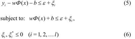
3. State Key Laboratory of Ocean Engineering, Shanghai Jiao Tong University, Shanghai 200240, China
4. Wuhan Second Ship Design and Research Institute, Wuhan 430064, China
System identification mo*delling of ship manoeuvring motion based onεsupport vector regression
WANG Xue-gang (王雪刚)1,2, ZOU Zao-jian (邹早建)1,3, HOU Xian-rui (侯先瑞)1, XU Feng (徐锋)4
1. School of Naval Architecture, Ocean and Civil Engineering, Shanghai Jiao Tong University, Shanghai 200240,China
2. CCCC Fourth Harbor Engineering Institute Co., Ltd., Guangzhou 510230, China, E-mail:510simon@163.com
3. State Key Laboratory of Ocean Engineering, Shanghai Jiao Tong University, Shanghai 200240, China
4. Wuhan Second Ship Design and Research Institute, Wuhan 430064, China
Based on the ε-support vector regression, three modelling methods for the ship manoeuvring motion, i.e., the white-box modelling, the grey-box modelling and the black-box modelling, are investigated. The10o/10o,20o/20ozigzag tests and the 35oturning circle manoeuvre are simulated. Part of the simulation data for the 20o/20ozigzag test are used to train the support vectors, and the trained support vector machine is used to predict the whole20o/20ozigzag test. Comparison between the simulated and predicted20o/20ozigzag test shows a good predictive ability of the three modelling methods. Then all mathematical models obtained by the modelling methods are used to predict the10o/10ozigzag test and 35oturning circle manoeuvre, and the predicted results are compared with those of simulation tests to demonstrate the good generalization performance of the mathematical models. Finally, the modelling methods are analyzed and compared with each other in terms of the application conditions, the prediction accuracy and the computation speed. An appropriate modelling method can be chosen according to the intended use of the mathematical models and the available data for the system identification.
ship manoeuvring, hydrodynamic coefficients, mathematical model, system identification,ε-support vector regression
Introduction
The ship manoeuvrability is explicitly required in the Standards for Ship Manoeuvrability promulgated by the International Maritime Organization[1]. To predict the ship manoeuvrability at the ship design stage,some methods are available, including the database and/or empirical formula method, the free-running model test method, the numerical method and the computer simulation method based on mathematical models. The last one is popular and effective to predict the ship manoeuvrability. To use this method, constructing accurately the mathematical model is a necessary precondition. The application of the system identification (SI) based on the free-running model tests or the full-scale trials plays an important role in modelling the ship manoeuvring motion.
Various classical SI methods, e.g., the extended Kalman filter method[2,3], the maximum likelihood method[4], the recursive prediction error method[5]and the least squares method[6], were applied in modelling the ship manoeuvring motion and identifying the hydrodynamic coefficients. However, they have some inherent defects, such as the sensitivity to the initial values, the ill-conditioned solutions and the simultaneous drift. To eliminate these defects, some modern SI methods were proposed for estimating the hydrodynamic coefficients, including the frequency domain identification method[7,8], the neural network[9], the su-pport vector machines (SVM)[10-13]and the genetic algorithm[14]. Among them, the neural network and the support vector machines, as two kinds of artificial intelligence algorithms, can not only be used for the parametric identification, but also, even more suitably,for the nonlinear regression. Rajesh and Bhattacharyya[15]adopted the artificial neural network to regress the nonlinear dynamic model of a large tanker. Moreira and Guedes Soares[16]applied the recursive neural network to simulate the ship manoeuvring motion. Compared with the neural network, the SVM is direct at finite samples and has better generalization performances and a global optimal extremum[17]. It is mainly used for pattern recognition and parameter identification. It is known as the support vector regression (SVR) when it is used for parameter identification. Luo and Zou[10,11], Zhang and Zou[12]identified the hydrodynamic coefficients in the Abkowitz model of the ship manoeuvring motion by using the least squares support vector regression (LS-SVR) and the ε-support vector regression (ε-SVR), respectively. The modelling method used in these two papers is only the white-box modelling, and to reduce the extent of parameter drift, a series of random signals is added into the training samples. However, the introduced random signal brings about another problem: the amplitude of the random signals is difficult to determine. Moreover, in order to obtain the hydrodynamic coefficients in the sway and yaw equations, it is necessary to solve a series of combined equations.
In the present paper, three modelling methods for the ship manoeuvring motion using the ε-SVR, i.e.,the white-box modelling, the grey-box modelling and the black-box modelling, are investigated. The whitebox modelling method is improved by reconstructing the identification formulas to avoid adding the random signals into the training samples and solving a series of combined equations. The grey-box modelling and the black-box modelling are clearly defined. The 10o/10o,20o/20ozigzag tests and the 35oturning circle manoeuvre are simulated by using the hydrodynamic coefficients obtained from the PMM test[18]. 5% of the simulation data of the 20o/20ozigzag test are used to train the support vectors, and the trained support vector machines are used to predict the whole 20o/20ozigzag test. The predicted results are compared with those of simulation tests to demonstrate the good predictive ability of the mathematical models obtained by the modelling methods. Then, the mathematical models are used to predict the 10o/10ozigzag test and the 35oturning circle manoeuvre, and the predicted results are compared with those of simulation tests to demonstrate the generalization performance of the mathematical models. The modelling methods are analyzed and compared with each other in terms of the application conditions, the prediction accuracy and the computation speed. An appropriate modelling method can be chosen according to the intended use of the mathematical models and the available data for the system identification.
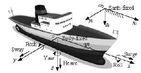
Fig.1 Coordinate systems
1. Mathematical model of ship manoeuvring motion
As shown in Fig.1, two right-handed coordinate systems, the earth-fixed inertial frame (the global coordinate system)o0-x0y0z0and the body-fixed moving frame (the local coordinate system)o-xyz , are adopted, with the plane o0-x0y0z0on the undisturbed free surface and z0-axis pointing downwards. At the initial instant, these two coordinate systems coincide with each other.
Generally, the manoeuvring motion of a surface ship can be described by the equations of the surge,sway and yaw motions in the following form[18]
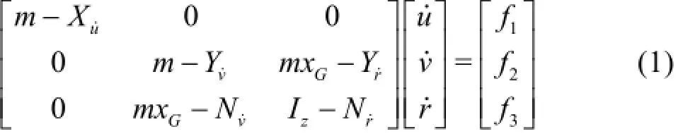
where
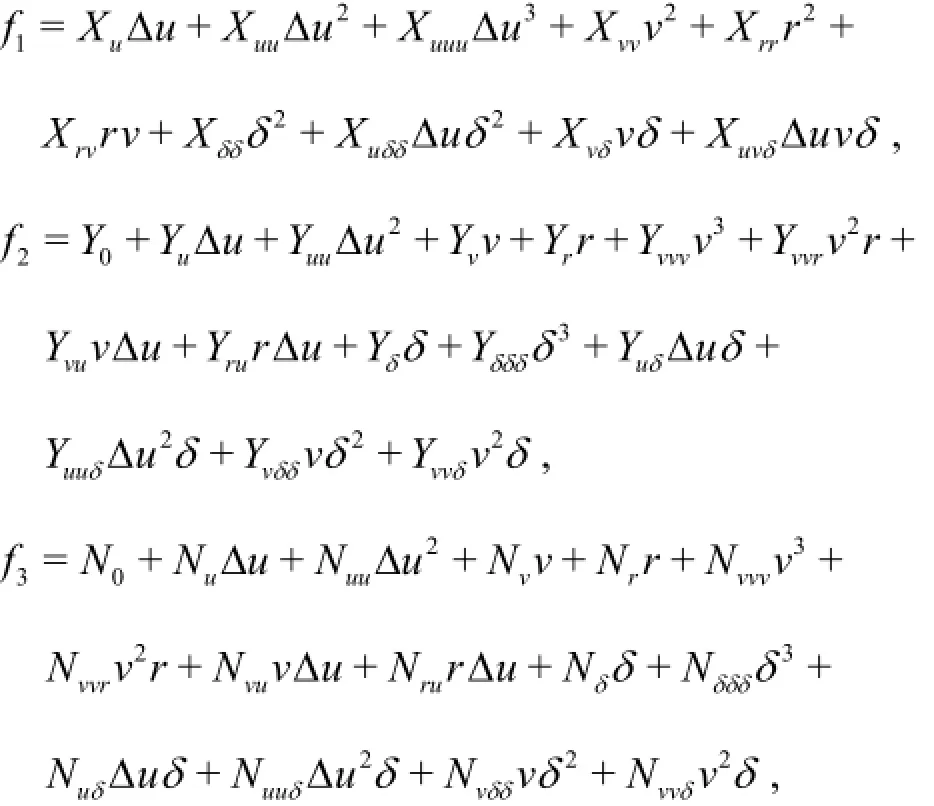
m is the mass of the ship,Izis the moment of inertia of the ship aboutz -axis and xGis the longitudinal coordinate of the ship gravity centre in the bodyfixed coordinate system,u,vandrare the surge speed, the sway speed and the yaw rate, respectively,δis the rudder angle,Δuis the disturbing quantity of the surge speed.Xu,Yv,Nretc. are the hydrodynamic coefficients,Y0and N0are the hydrodynamic force in the direction of y-axis and the yaw moment aboutz-axis during the straight forward motion with constant speed.
Denoting the kinetic parameters at the state of the straight forward motion with constant speed by subscript 0, we have u0=U0,Δu=u-u0,v0=r0=δ0===˙=0. The resultant speedU=[(u0+ Δu)2+v2]1/2.
2.ε-support vector regression
Based on the statistical learning theory, the SVM is effective to improve the generalization performance and can be used to obtain the globally optimal and unique solution[17]. Initially, the SVM was applied in the area of pattern recognition, with the introduction of the insensitive loss function, the SVM was extended to solve non-linear regression estimations,known as the support vector regression (SVR).
The main idea of the SVR is to map the input data into a high-dimensional feature space and to do linear regression in this space. The optimum regression function can be described as

wherexandy are the input and output vectors of the system, respectively, and they are defined in the high-dimensional feature space,Φ(x)represents the high-dimensional feature space, which is nonlinearly mapped from the input spacex,wis the weight matrix,b is the bias,R is the Euclidean space,l andn are the dimensions of the Euclidean space.
The SVR aims to find a function that represents the deviation ofεfrom the actual output. The coefficientswandb are estimated by minimizing the regularized risk function:
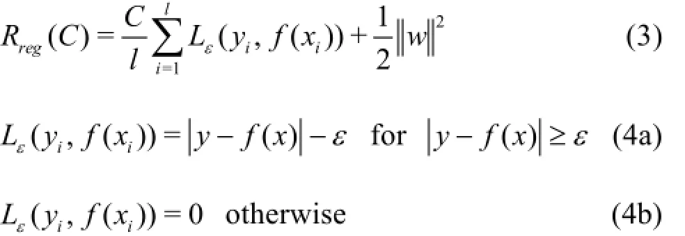
Introducing the slack variablesandinto Eqs.(3) and (4), they are transformed to form the dual optimization problem: minimize:
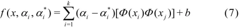
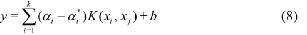
To avoid computing explicitly the mapping Φ(x), introducing K(xi,xj)=Φ(xi)Φ(xj)in Eq.(7),K(xi,xj)is known as the kernel function, it follows that
Any function that satisfies the Mercer condition can be used as the kernel function. Some commonly used kernel functions are: (1) the linear kernel function, (2) the polynomial kernel function, (3) the RBF kernel function, (4) the sigmoid kernel function, and(5) the B-spline kernel function.
3. System identification modelling
The SI combined with the free-running model tests or the full-scale trials is one of the effective methods for modelling the ship manoeuvring motion. There are three kinds of SI modelling, including the white-box modelling, the grey-box modelling and the black-box modelling. The white-box modelling is also known as the mechanism modelling. In the white-box modelling, the motion of the system is analyzed based on the structure of the system; and the mathematical model of the system is built. The black-box modelling is a modelling method that uses only the input-output data of the system, even if both the structure and the parameters of the system are unknown. It aims to obtain an appropriate approximation of the actual system. The grey-box modelling is a hybrid modelling method combining the white-box modelling and the black-box modelling for the system that is not fully known.
3.1White-box modelling
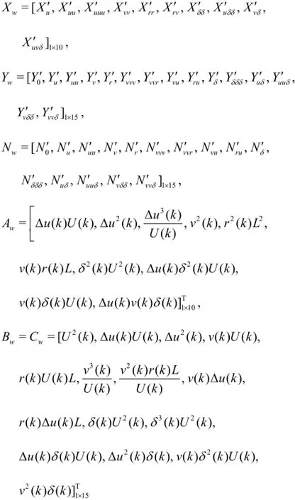
In the white-box modelling, the mathematical model structure of the objective ship, the principal parameters of the ship and the acceleration derivatives in the mathematical model are known. Firstly, the Lagrangian multipliers are trained by using the samples of the input and output to identify the hydrodynamic coefficients; secondly, the ship manoeuvring motion is predicted with the identified hydrodynamic coefficients and Eqs.(1)-(4).
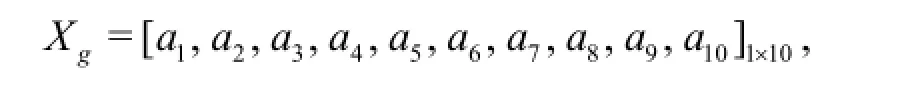
In the process of identification, the parameter drift happens inevitably. How to reduce the parameter drift is vital to the identification accuracy of the hydrodynamic coefficients. To reduce the extent of the parameter drift, Luo and Zou[10], Zhang and Zou[12]added a series of random signals into the training samples. However, the introduction of the random signals brings about another problem: the amplitude of the random signals is difficult to determine. Moreover, to obtain the hydrodynamic coefficients in the sway and yaw equations, it is necessary to solve a series of combined equations. In the present work, the identification formulas are reconstructed to avoid adding the random signals into the training samples and solving a series of combined equations. First of all, the continuous equation of motion is discretized using Euler's stepping method as
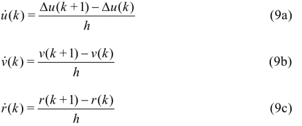
whereh is the sampling interval,kand k +1are the adjacent sampling time steps.
Substituting Eq.(9) into Eq.(1), the reconstructed identification formulas are obtained as

where L is the ship length, and the coefficient vectors and the variable vectors are
Note that in order to facilitate the identification, the motion state parameters (U,u,v,randδ) maintain in the dimensional form in Eq.(10), while the hydrodynamic coefficients are written in the non-dimensional form[18].
The above coefficient vectors can be identified by using the ε-SVR. Here the linear kernel function K(x,x′)=xx′is selected and Eq.(8) is rewritten as

Comparing Eq.(10) with Eq.(11), if the ε-SVR can provide a good approximation of the objective function (which means thatb is infinitely close to zero),are the identified hydrodynamic coefficients.
The detailed process of the white-box modelling and the prediction of the ship manoeuvring motion using the ε-SVR is depicted in Fig.2.
Fig.3 Process of grey-box modelling using ε-SVR
3.2Grey-box modelling
If it is not necessay to know the hydrodynamic coefficients apart from the prediction of the ship manoeuvring motion, the grey-box modelling is a better choice. In this case, only the structures of the mathematical model are known, while other information,even the ship's principal particulars, is unknown. In the grey-box modelling, the support vectors are firstly trained by using the samples of the input and output,and then the ship manoeuvring motion is predicted by using the trained support vectors, without using Eq.(1).

Table 1 Main particulars of mariner class vessel
Substituting Eq.(9) into Eq.(1), the output can be rearranged as:
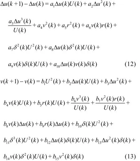
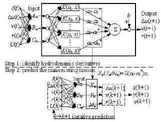
Fig.2 Process of white-box modelling using ε-SVR
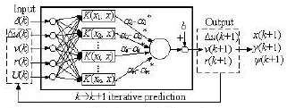
Fig.4 Process of black-box modelling using ε-SVR
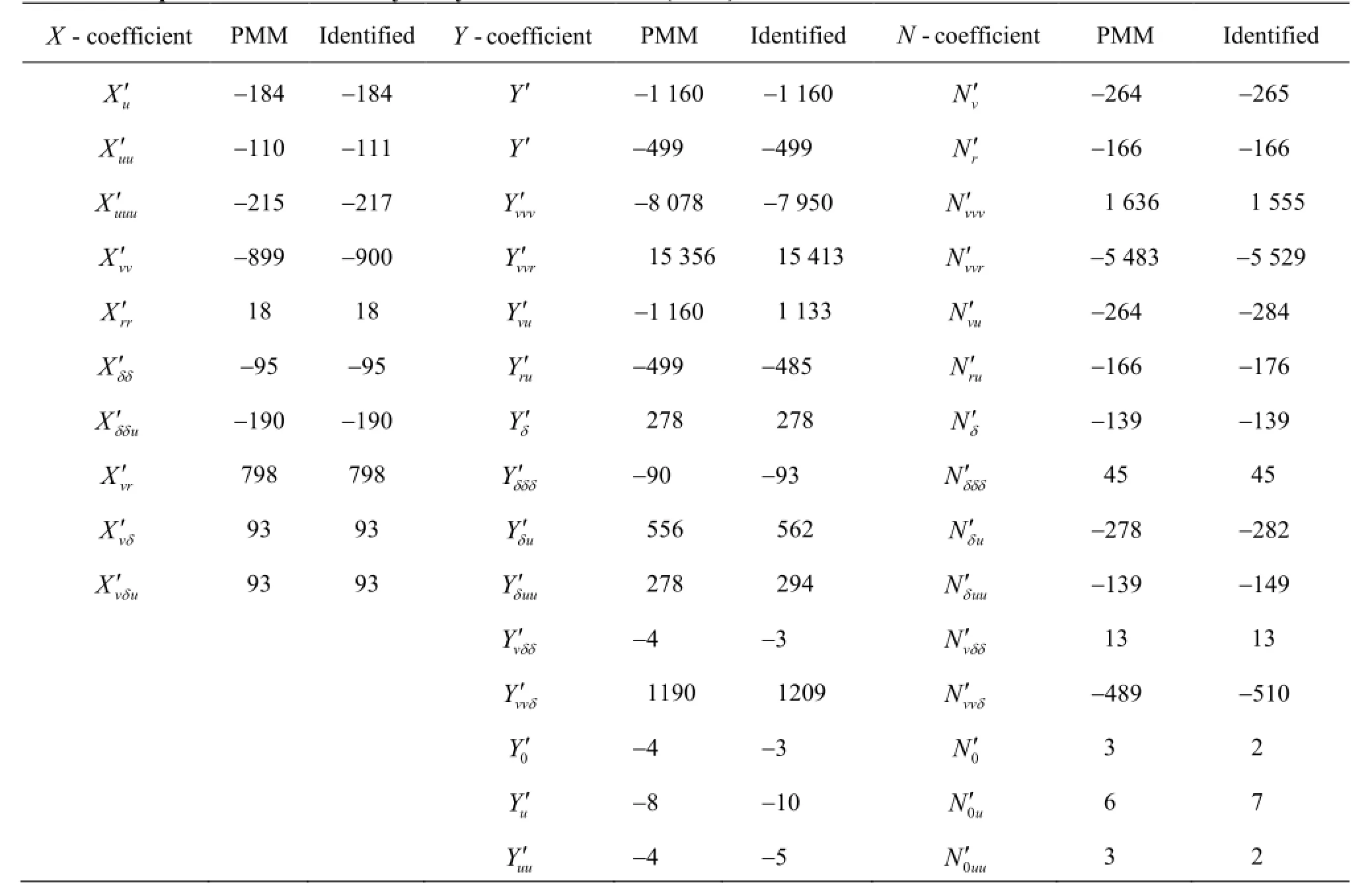
Table 2 Comparison of identified hydrodynamic coefficients (×10-5) with PMM test data
where the coefficient vectors and the variable vectors are
The process of the grey-box modelling and the prediction of the ship manoeuvring motion using the ε-SVR is depicted in Fig.3.
3.3Black-box modelling
When neither the ship's principal parameters, nor the structures of the mathematical model are known,the black-box modelling is the only choice for modelling the ship manoeuvring motion. In the black-box modelling, only the motion state variables at the last time step are used to predict those at the next time step.
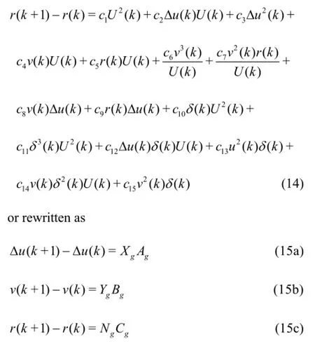
From Eqs.(12)-(14), it can be seen that Δu(k+1),v(k +1)and r(k +1)are functions of U(k),Δu(k),v(k),r(k )and δ(k). These equations can be rewritten as
The process of the black-box modelling and the prediction of the ship manoeuvring motion using ε-SVR is depicted in Fig.4.
4. Prediction and generalization verification
4.1Prediction
A Mariner Class Vessel[18]is taken as the study object. Table 1 gives the main particulars of the ship. The non-dimensional mass of the ship m′=7.98× 10⁻³, the non-dimensional moment of inertia of the ship about z-axis′=3.92×10⁻⁴and the non-dimensional longitudinal coordinate of the ship's centre of gravity-2.3×10⁻².
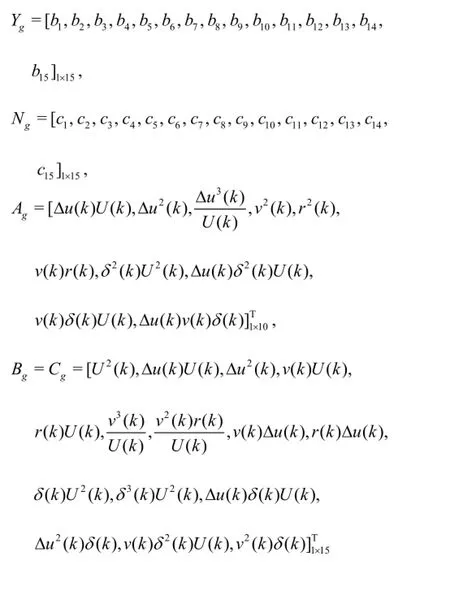
The 10o/10o,20o/20ozigzag tests and the 35oturning circle manoeuvre are simulated by using the hydrodynamic coefficients obtained from the PMM test[18], as given in Table 2. The zigzag tests are terminated after the rudder execution has repeated 5 times,for the turning circle manoeuvre, the rudder is deflected to the desired angle and maintains until the heading of the ship has changed by 540o. The time histories of the surge speedu , the sway speedv , the yaw rater , the resultant speedU and the heading angle ψare obtained from the simulation. The simulation sampling interval is 0.2 s.
In the identification process, the simulation data of the 20o/20ozigzag test are used to identify the hydrodynamic coefficients. The white Gaussian noise is added to the simulation data of the surge speed, the sway speed, the yaw rate and the heading angle as the observation values, and then the data with noise are filtered with the wavelet denoising method. Figure 5 shows the comparison of the original simulation data,the simulation data with white Gaussian noise and the denoised data.
The training sample couples are taken from the denoised simulation data of the 20o/20ozigzag test every 4 s (5% of the denoised simulation data). The penalty factor C =106and the insensitivity factor ε=10-6are chosen.
In the white-box modelling, the training sample couples consist of
input:{Aw,Bw,Cw}
Fig.5 Comparison of the 20o/20ozigzag test data

Fig.6 Comparison of the predicted motions with simulation results,20o/20ozigzag test
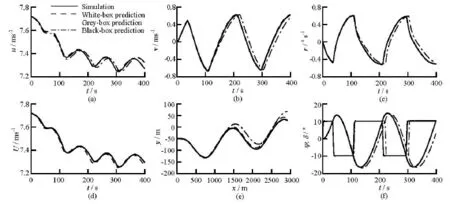
Fig.7 Comparison of the predicted motions with simulation results,10o/10ozigzag test

The hydrodynamic coefficients are identified by Eq.(11) and the results are given in Table 2 in comparison with the data obtained from the PMM test. Note that the acceleration derivatives are not identified and are treated as known constants during identification.
It can be seen from Table 2, the identification results of the hydrodynamic coefficients are in good agreement with the PMM test data, which indicates that the white-box modelling using the ε-SVR is an effective method to identify the hydrodynamic coefficients.
In the grey-box modelling, a linear kernel function is selected. The training sample couples consist of
input:{Ag,Bg,Cg}
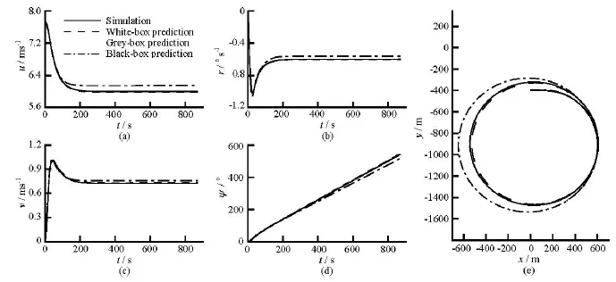
Fig.8 Comparison of the predicted motions with simulation results,35oturning circle manoeuvre
output:{Δu(k+1)-Δu(k),v(k+1)-v(k),
In the black-box modelling, the RBF kernel functionis selected, with the width parameterσ=20. The training sample couples consist of
input:{U(k),Δu(k),v(k),r(k),δ(k)}
output:{Δu(k+1)-Δu(k),v(k+1)-v(k),
Figure 6 shows the predicted motions of the 20o/20ozigzag test using the mathematical models obtained by the white-box modelling, the grey-box modelling and the black-box modelling in comparison with those of simulation data with noise. A satisfactory agreement demonstrates the validity of the proposed identification modelling methods.
4.2Generalization verification
To verify the generalization performance of the modelling methods, the 10o/10ozigzag test and the 35oturning circle manoeuvre are predicted by using the support vectors trained with the denoised simulation data of the20o/20ozigzag test. The comparisons of the predicted motions with the simulation results are shown in Fig.7 and Fig.8. As it can be seen from these figures, good agreements are achieved, which demonstrates that the modelling methods have a good generalization capability.
4.3Comparison
The requirements of the known conditions and the output results of the three modelling methods are listed in Table 3. According to the intended use of the mathematical models and the available data needed for the system identification, an appropriate modelling method can be chosen. If the hydrodynamic coefficients are to be determined, the white-box modelling might be chosen, however, many known data are required in the white-box modelling. When only the structures of the mathematical models are known, the grey-box modelling is a better choice. When neither the ship's principal parameters, nor the structures of the mathematical models are known, the black-box modelling is the only choice.
Usually, the mean square error (MSE) and the correlation coefficient (CC) are two evaluation criteria used to measure the prediction accuracy. Taking the surge speed(u)as an example, the MSE and the CC are defined as:
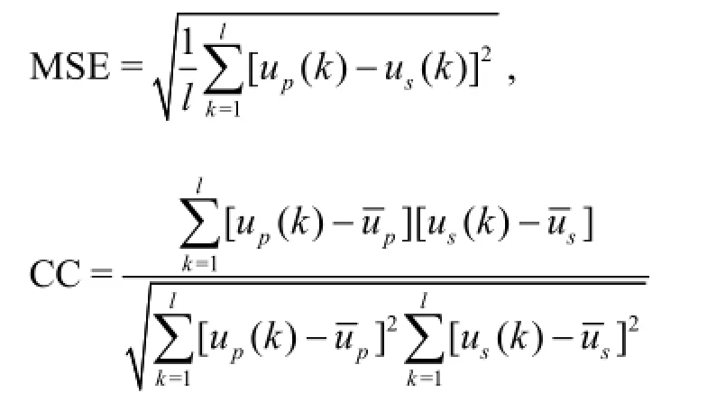
where the subscriptpands denote the prediction result and the simulation result, respectively,l is the number of the surge speed data,anddenote the average prediction result and the simulation result,respectively.

Table 3 Requirements of known conditions and output of the modelling methods
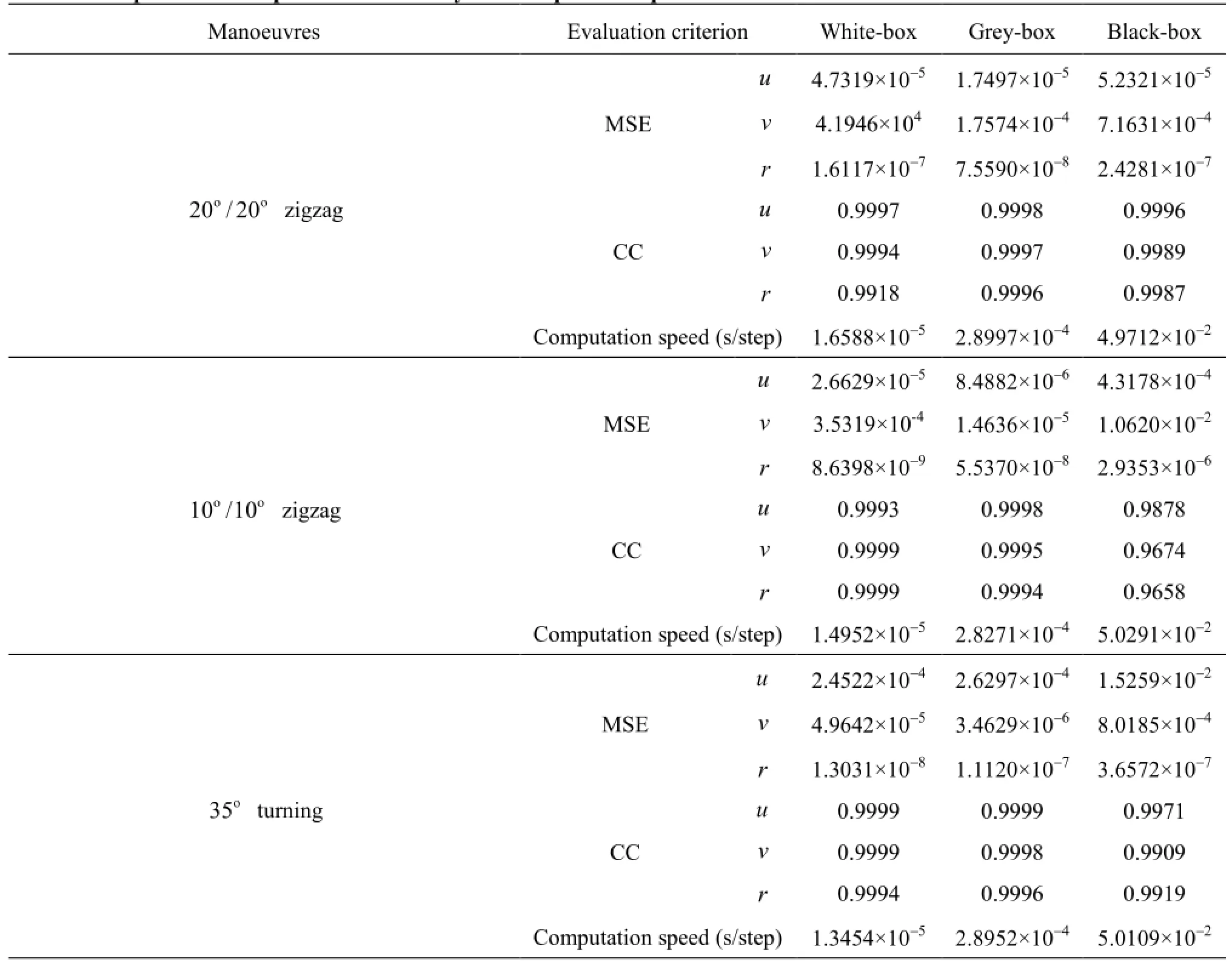
Table 4 Comparison of the prediction accuracy and computation speed
The MSE and the CC ofu,vandrare listed in Table 4, where the computation speed is also shown. All predictions using the mathematical models obtained by the modelling methods are made under the same computation condition and software environment.
Table 4 demonstrates that all modelling methods have a high prediction accuracy. However, the accuracy of the white-box modelling and the grey-box modelling is significantly higher than that of the blackbox modelling. It is because the inputs of the whitebox modelling and the grey-box modelling are bothhigh-dimensional vectors and hence can better reflect the system characteristics; while the input of the black-box modelling is only one-dimensional vector. The white-box modelling and the grey-box modelling have a stronger nonlinear mapping ability than the black-box modelling, although the RBF kernel function is chosen in the black-box modelling.
Table 4 also demonstrates that all modelling methods have a fast computation speed. However, the white-box modelling takes much less computation time than the grey-box modelling and the black-box modelling. In the white-box modelling, the ship manoeuvring motion is predicted with the identified hydrodynamic coefficients and the mathematical model(Eq.(1)), and hence is the fastest. In the grey-box modelling and the black-box modelling, the ship manoeuvring motion is predicted by using the trained support vectors, without the use of the mathematical model. The prediction based on the grey-box modelling involves a high dimensional nonlinear input, and hence takes a large amount of computation time. Although the input of the black-box modelling is very simple,the high-dimensional kernel function such as the RBF kernel function requires quite large memory and CPU time.
5. Conclusions
Based on the ε-SVR, this paper studies three system identification modelling methods for the ship manoeuvring motion, i.e., the white-box modelling,the grey-box modelling and the black-box modelling. The conclusions can be summarized as follows:
(1) Good predictive ability and generalization performance of the modelling methods are demonstrated by comparing the predicted results with those of simulation tests.
(2) An appropriate modelling method can be chosen according to the intended use of the mathematical models and the available data for the system identification. When the hydrodynamic coefficients are to be determined, the white-box modelling might be chosen,when only the structures of the mathematical models are known, the gray-box modelling is a better choice,when neither the ship's principal parameters, nor the structures of the mathematical models are known, the black-box modelling is the only choice.
(3) By comparing the MSE and the CC between the predicted results and the simulation data, it is shown that the accuracy of the white-box modelling and the grey-box modelling is significantly higher than that of the black-box modelling.
(4) It is shown that all modelling methods have a fast computation speed, because of theε-SVR characteristics. In comparison, the white-box modelling requires much less computation time than the grey-box modelling and the black-box modelling.
References
[1]IMO. Standards for ship manoeuvrability[S]. Resolution MSC.137(76), International Maritime Organization(IMO), 2002.
[2]ABKOWITZ M. A. Measurement of hydrodynamic characteristic from ship maneuvering trials by system identification[J]. Transactions of Society of Naval Architects and Marine Engineers, 1980, 88: 283-318.
[3]HWANG W. Y. Application of system identification to ship maneuvering[D]. Doctoral Thesis, Boston, USA:Massachusetts Institute of Technology, 1980.
[4]ÅSTRÖM K. J., KÄLLSTRÖM C. G. Identification of ship steering dynamics[J]. Automatica, 1976, 12(1): 9-22.
[5]ZHOU W. W., BLANKE M. Identification of a class of nonlinear state-space models using RPE techniques[J]. IEEE Transactions on Automatic Control, 1989, 34(3):312-316.
[6]RHEE K. P., LEE S. Y. and SUNG Y. J. Estimation of manoeuvring coefficients from PMM test by genetic algorithm[C]. Proceedings of International Symposium and Workshop on Force Acting on a Manoeuvring Vessel. Val de Reuil, France, 1998, 77-87.
[7]BHATTACHARYYA S. K., HADDARA M. R. Parametric identification for nonlinear ship manoeuvring[J]. Journal of Ship Research, 2006, 50(3): 197-207.
[8]PEREZ T., FOSSEN T. I. Practical aspects of frequencydomain identification of dynamic models of marine structures from hydrodynamic data[J]. Ocean Engineering,2011, 38(2-3): 426-435.
[9]HADDARA M. R., WANG Y. Parametric identification of manoeuvring models for ships[J]. International Shipbuilding Progress, 1999, 46(445): 5-27.
[10]LUO W., ZOU Z. Parametric identification of ship maneuvering models by using support vector machines[J]. Journal of Ship Research, 2009, 53(1): 19-30.
[11]LUO Wei-lin, ZOU Zao-jian. Elimination of simultaneous drift and sensitivity analysis in the hydrodynamic modeling of ship manoeuvring[J]. Journal of Shanghai Jiaotong University, 2008, 42(8): 1358-1362(in Chinese).
[12]ZHANG Xin-guang, ZOU Zao-jian. Identification of Abkowitz model for ship manoeuvring motion using ε-support vector regression[J]. Journal of Hydrodynamics, 2011, 23(3): 353-360.
[13]XU Feng, ZOU Zao-jian and YIN Jian-chuan et al. Parametric identification and sensitivity analysis for autonomous underwater vehicles in diving plane[J]. Journal of Hydrodynamics, 2012, 24(5): 744-751.
[14]SUTULO S., GUEDES SOARES C. An algorithm for offline identification of ship manoeuvring mathematical models from free-running tests[J]. Ocean Engineering,2014, 79: 10-25.
[15]RAJESH G., BHATTACHARYYA S. K. System identification for nonlinear maneuvering of large tankers using artificial neural network[J]. Applied Ocean Research,2008, 30(4): 256-263.
[16]MOREIRA L., GUEDES SOARES C. Dynamic model of manoeuvrability using recursive neural networks[J]. Ocean Engineering, 2003, 30(13): 1669-1697.
[17]VAPNIK V. N. The nature of statistical learning theory[M]. New York, USA: Springer Verlag, 2000.
[18]FOSSEN T. I. Handbook of marine craft hydrodynamics and motion control[M]. New York, USA: John Wiley and Sons, 2011.
(March 17, 2014, Revised October 31, 2014)
* Project supported by the National Natural Science Foundation of China (Grant No. 51279106), the Special Research Fund for the Doctoral Program of Higher Education of China(Grant No. 20110073110009).
Biography: WANG Xue-gang (1983-), Male, Ph. D.
ZOU Zao-jian,
E-mail: zjzou@sjtu.edu.cn
杂志排行

水动力学研究与进展 B辑的其它文章
- The analysis of flow characteristics in multi-channel heat meter based on fluid structure model*
- The gas recovery of water-drive gas reservoirs*
- Advances of drag-reducing surface technologies in turbulence based on boundary layer control*
- A review of studies of mechanism and prediction of tip vortex cavitation inception*
- Propulsive performance of a passively flapping plate in a uniform flow*
- Numerical analyses of pressure fluctuations induced by interblade vortices in a model Francis turbine*