The gas recovery of water-drive gas reservoirs*

LI Min （李闽）， LI Tao （李滔）， JIANG Qiong （蒋琼）， YANG Hai （杨海）， LIU Shi-chang （刘世常）

State Key Laboratory of Oil and Gas Reservoir Geology and Exploitation， Southwest Petroleum University，Chengdu 610500， China， E-mail： hytlxf@126.com

The gas recovery of water-drive gas reservoirs*

LI Min （李闽）， LI Tao （李滔）， JIANG Qiong （蒋琼）， YANG Hai （杨海）， LIU Shi-chang （刘世常）

State Key Laboratory of Oil and Gas Reservoir Geology and Exploitation， Southwest Petroleum University，Chengdu 610500， China， E-mail： hytlxf@126.com

This paper proposes a method for determining the gas recovery of water-drive gas reservoirs. First， the water influx coefficientB in the theoretical formula=（1-）/（1-）is used to determine the influence of the aquifer behavior. According to the theoretical formula， the relationship between the normalized pressure prand the degree of the reserve recovery Rgcan be obtained with different values of B ， which can be used to determine the activity level of the aquifer behavior. Second，according to pra=（1-Rga）/（1-aEva）（where a=1-Sgr/Sgi）， the relationship between the normalized abandonment pressure praand the ultimate gas recovery Rgacan be obtained， as the Agarwal end-point line. The intersection of the above two lines represents the value of the estimated ultimate gas recovery and the normalized abandonment pressure pra. Finally， an evaluation table and a set of demarcation charts are established， with different values of Sgr/Sgiand Evaas well as the water influx coefficient B ， which can be used to determine the gas recovery of water-drive gas reservoirs with different activity levels of the aquifer behavior.

water-drive gas reservoirs， degree of reserve recovery， water influx coefficient， evaluation table， demarcation charts

Introduction

In the field of gas reservoir engineering， it is of great importance to determine the gas recovery of water-drive gas reservoirs， for a better understanding of the factors that affect the gas recovery and for a more effective way to enhance it. However， very few methods are available to determine the gas recovery of water-drive gas reservoirs. This paper proposes a graphical solution to this problem.

Agarwal et al. （1965） and El-Ahmady and Wattenbarge［1］demonstrated the effect of the water influx on the relationship between p/z and the cumulative gas production. They also illustrated that the effect was related to the lowered reservoir pressure. Furthermore， the ultimate gas recovery might be increased via retarding the water invasion. Agarwal et al.（1965） concluded that the gas recovery depends on the production rate， the residual gas saturation， the aquifer strength， the aquifer permeability and the volumetric sweep efficiency of the water invaded zone. The water influx could be monitored and determined by the methods of Glegola et al.［2］and Hu et al.［3］.

Pujiastuti and Ariadji［4］used a 2-D radial， 2-phase water-gas flow model to study the relationship between the residual gas saturation and the recovery of water-drive gas reservoirs. Meanwhile， the recovery of the water-drive gas reservoirs could be predicted from the knowledge of the residual gas saturation and the abandonment pressure. It is shown that the gas recovery is affected by the aquifer strength and the heterogeneity， as is consistent with Agarwal's （1965）. Sheng［5］studied the effect of 3 univariate gas reservoir geological parameters on the gas reservoir development， which was shown to be mainly determined by the permeability and the porosity.

Papay［6］and Holtz［7］， respectively， introduced the correlation method and the calculation method for a 3-D computer reservoir model to calculate the residual gas saturation. Furthermore， residual gas saturation experiments of water-drive gas reservoirs were carried out［8，9］. The results indicated that the residual gas saturation was related to the initial gas saturation，which was also consistent with Suzanne et al.［10］. In addition， Le et al.［11］studied the impact of the capillarity on the gas recovery for tight sands. Khan et al.［12］and Hughes et al.［13］introduced methods of CO2injection and CO2sequestration to improve the gas recovery， with significant effects.

Li and Hao［14］used an improved volume method to calculate the gas recovery， to correct the error of the original volume method in calculating the geological reserve， and with consideration of the difference of the gas saturation of different reservoirs. Based on experiment and production data， Wu et al.［15］proposed a new empirical formula to predict the recovery of condensate gas reservoirs， specially for ones in China， where the condensate oil content is less than 400 g/m3and the abandoned pressure is about 3.4 MPa.

To sum up， among many methods proposed to determine the recovery of water-drive gas reservoirs，there is few with a clear basis and reliability. Meanwhile， existing charts and tables for the determination of the recovery are based on the field data without a definite theoretical basis， and their extensive use might not be reliable.

In this paper， a kind of graphical solution is proposed to determine the gas recovery based on the empirical formulae of water-drive gas reservoirs. Moreover， an evaluation table and a set of recovery demarcation charts are developed.

1. Theoretical curves and theoretical equation

In the study of the relationship between the water influx coefficientB and the degree of the reserve recovery Rg， Zhang and Li［16］found that， in many cases，ωhas a logarithmic relationship with Rg. This can be expressed in the mathematical form as

whereωis defined by the following expression［17］

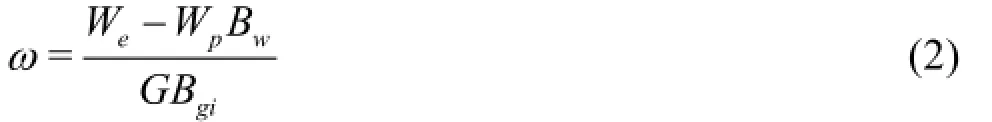
whereωis the remaining water coefficient，Bwis the water volume factor andBgiis the gas volume factor under the initial formation condition. The subscriptw refers to the water， the subscriptg refers to the gas and the subscripti refers to the initial condition.Weis the cumulative water influx volume and Wpis the cumulative water production volume.

Equation （1） can also be written as

The value ofBdecreases as the water influx increases， and vice versa. Ignoring the water and rock compressibility， the material balance equation of water-drive gas reservoirs can be established， as

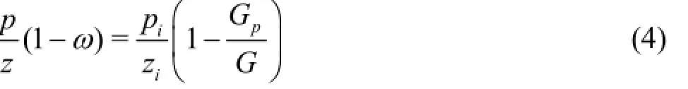
wherep is the pressure，piis the initial formation pressure andGpis the cumulative gas production at timet.

Set pr=（p/z）/（pi/zi）［16］， which is called the normalized p/z . Since Rg=Gp/G， Eq.（4） can be expressed as

Equation （5） gives a relationship between prand RgwhenBis given or can be estimated， which can serve as a theoretical basis， therefore， Eq.（5） is referred to as the theoretical formula. Different values of Bcorrespond to different theoretical curves as shown in Fig.1.

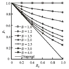
Fig.1 Theoretical curves

2. Aquifer behavior

Equrtion （1） indicates we will have a rigid waterdrive gas reservoir whenB is equal to 1.0， whichmeans that the power of the aquifer could keep the formation pressure in its original state. WhenB→∞and ω→0， we have a gas reservoir without water invading. When1＜B＜∞， we have a common waterdrive reservoir. If B≥4， the strength of the water influx is rather weak， thus the effect of the water influx on the gas production performance can be ignored. So we just study the gas recovery and the aquifer behavior in the range1＜B＜4.

Zhang and Li［16］found thatB could be regarded as a constant if the production strategy does not change greatly， and one of the theoretical curves would approximately match the reservoir performance. For a specific reservoir， the curve of prvs.Rgcan be obtained when a certain values of prand Rgare given， which usually can be calculated from the production and testing data. The curve of prvs.Rgrefers to the field normalized p/z curve as shown in Fig.2 （solid line）.

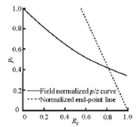
Fig.2 Field normalized p/z curve and normalized end-point line

As mentioned previously， there must be one theoretical curve approximately reflecting the reservoir production performance， which also should very closely match the field normalized p/z curve. However， the field normalized p/z curve can only be obtained by the field production and testing data after the reservoir is abandoned. Therefore， the approximately-matched theoretical curve is more appropriate to be adopted to determine the activity level of the aquifer behavior.

According to the classification proposed by Zhang and Li［16］， the aquifer behaviors are classified into three grades， i.e.，1＜B＜1.5，1.5＜B＜2.5and 2.5＜B＜4， with a large recovery error. In this paper，in terms of the aquifer behavior， the water-drive gas reservoirs are classified into six grades： the active grade I， when 1＜B＜1.2， the active grade II， when 1.2＜B＜1.5， the moderate grade I， when 1.5＜B＜2，the moderate grade II， when 2＜B＜2.5， the inactive grade I， when 2.5＜B＜3， the inactive grade II， when 3＜B＜4（See Table 1）. Based on this classification，the theoretical curves are established as shown in Fig.1 and the recovery range of each grade can be kept within 10% or so. Now， if we put the values of prand Rgor the field normalized p/z curve on Fig.1，the values or the curve might locate in one of the six influx areas on the chart. According to the classification mentioned above， the activity level of the aquifer behavior of the gas reservoir can be determined.

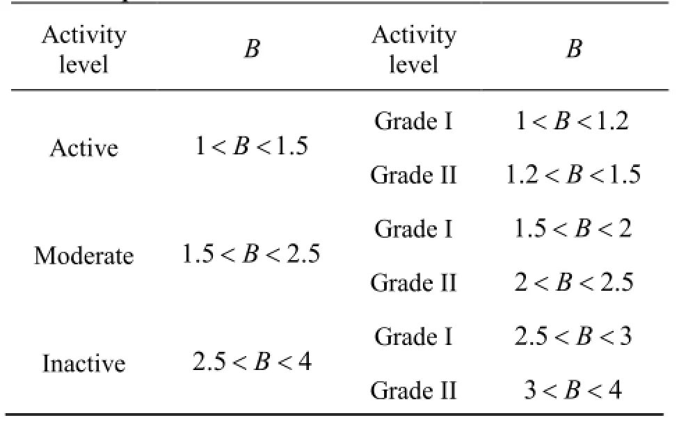
Table 1 Aquifer behavior level classification

3. Method

3.1Normalized end-point formula and normalized end-point line

When the end point （pa/za）is determined， or under the abandonment condition， the residual gas is comprised of the trapped gas and the unswept gas. The cumulative gas production under the abandonment condition Gpais equal to the initial gas-in-place（G）minus the trapped and unswept gas volume（Agarwal et al. （1965））. Agarwal end-point formula is

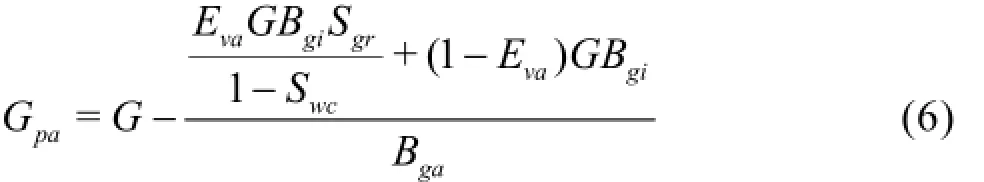
The subscripta refers to the abandonment condition，Bgais the gas volume factor under the abandonment condition and Evarefers to the volumetric sweep efficiency. In terms of the pressure， Eq.（6） can be expressed as in the following formula （Agarwal et al.（1965））

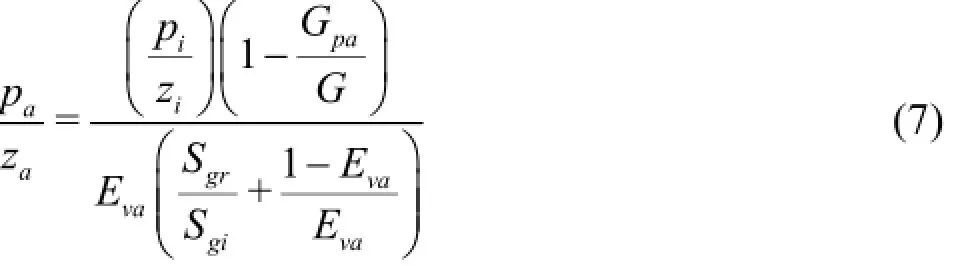
In this form， it is clear that Eq.（7） expresses the end point （pa/za）as a linear function of the gas recovery （Rga=Gpa/G）under the abandonment condition.

So Eq.（7） can be rearranged as

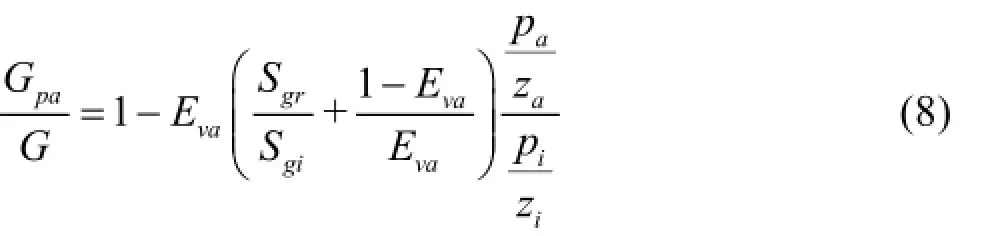
Herez is the gas deviation factor，ziis the gas deviation factor under the initial formation condition and zais the gas deviation factor under the abandonment condition.

Equation （7） can be simplified as

where

Equation （9） is called the normalized end-point formula which covers all values of praand Rgawith aEvagiven for a specific gas reservoir.praand Rgaare replaced by prand Rg， respectively. The field production data （prand Rg） are plotted on the same chart based on the relationship of Eq.（9）. Then Eq.（9）can be expressed as a linear formula， and is called the normalized pseudo-end-point formula with two unknowns prand Rg

Equation （10） suggests that if Rgis plotted against prwhenaand Evaare given， we will have a straight line which is called the normalized end-point line （dashed line in Fig.2）.There is only one credible point on this line due to the fact that only one pair of praand Rgaexists for a specific gas reservoir.

3.2Residual gas saturation and ultimate volumetric sweep efficiency

Notice that the values ofaand Evaare indispensable for the normalized end-point line. The value of a （a=1-Sgr/Sgi）can be obtained if Sgr/Sgiis known. After 320 experimental measurements，Agarwal （1965） proposed some formulae to calculate Sgrwith consideration of the effect of porosity and absolute permeability. In this paper， we adopt the Agarwal's formulae to calculate Sgr.

For cemented sandstones

where

A1=0.80841168，A2=-0.0063869116

For uncemented sandstones

where

For carbonate rocks

where

For cemented sandstones， based on the statistics of the data from 18 gas fields obtained by Zhang（1984） and Jin et al. （1987）， we propose that the irreducible water saturation Swcranges from 10% to 50% approximately， which is consistent with Roehl and Choquette's statistics （1985）. Thus it may be deduced that the range of the initial gas saturation Sgiis from 50% to 90% for general cases according to the statistical results. Then for cemented sandstones， the values of Sgrand Sgr/Sgican be calculated with Eq.（11） and the results are shown in Table 2， which indicates that the value of Sgr/Sgiranges from 0.2 to 0.5 when Sgiranges from 50% to 90%.

For uncemented sandstones， it is commonly known that Sgris a function of the porosity. He （1994）showed that the porosity ranges from 5% to 30% forsandstones， while for uncemented sandstones， the porosity is larger than 20%. So we let φ=20%，φ= 25% and φ=30%， respectively， to see the corresponding variation ofSgr/Sgi. In addition， the initial gas saturationSgifor uncemented sandstones still ranges from 50% to 90%. Table 2 shows the values ofSgrand Sgr/Sgifor uncemented sandstone and the ratio ofSgr/Sgiis from 0.1 to 0.4 while Sgiis from 50% to 90% andφis from 20% to 30%.

Table 2 Values of Sgr/Sgifor cemented and uncemented sandstones

Table 3 Values of Sgr/Sgiwith different kandφ

For carbonate rocks， from Eq.（13）， the residual gas saturation is a function of the porosity（φ）and the permeability（k ）. So it is necessary to study the corresponding properties of the porosity and the permeability. It is known that most reservoirs of Volga-Ural are distributed in Bashkir Strata in the former Soviet Union， where the porosity generally ranges from 10% to 20%. However， the porosity range of Duo Linna carbonate rocks in North Ukraine is from 13% to 16%， and the porosity of carbonate rocks ranges from 2.5% to 18% for many reservoirs with both matrix pores and fracture systems in the region of Belarus and Perm. Based on the statistical results， the range of the porosity we adopt for carbonate rocks is from 2.5% to 20%.

Petroleum reservoirs have the primary permeability， which is also known as the matrix permeability，and the secondary permeability. It is known that the range of the permeability for the reservoir rocks is mainly from 5 to 1 000 mD （He （1994）） and the logarithmic value of the permeability ranges from 0.7 to 3. For carbonate rocks， the value of the initial gas saturation Sgiranges from 50% to 90%. Thus， the range of Sgrcan be obtained according to Eq.（13）. Table 3 gives the values ofSgrand Sgr/Sgiwith different permeabilities， porosities andSgi. Meanwhile， it is also shown thatSgr/Sgiranges from 0.2 to 0.6 when Sgi=50%-90%，φ=2.5%-20%.

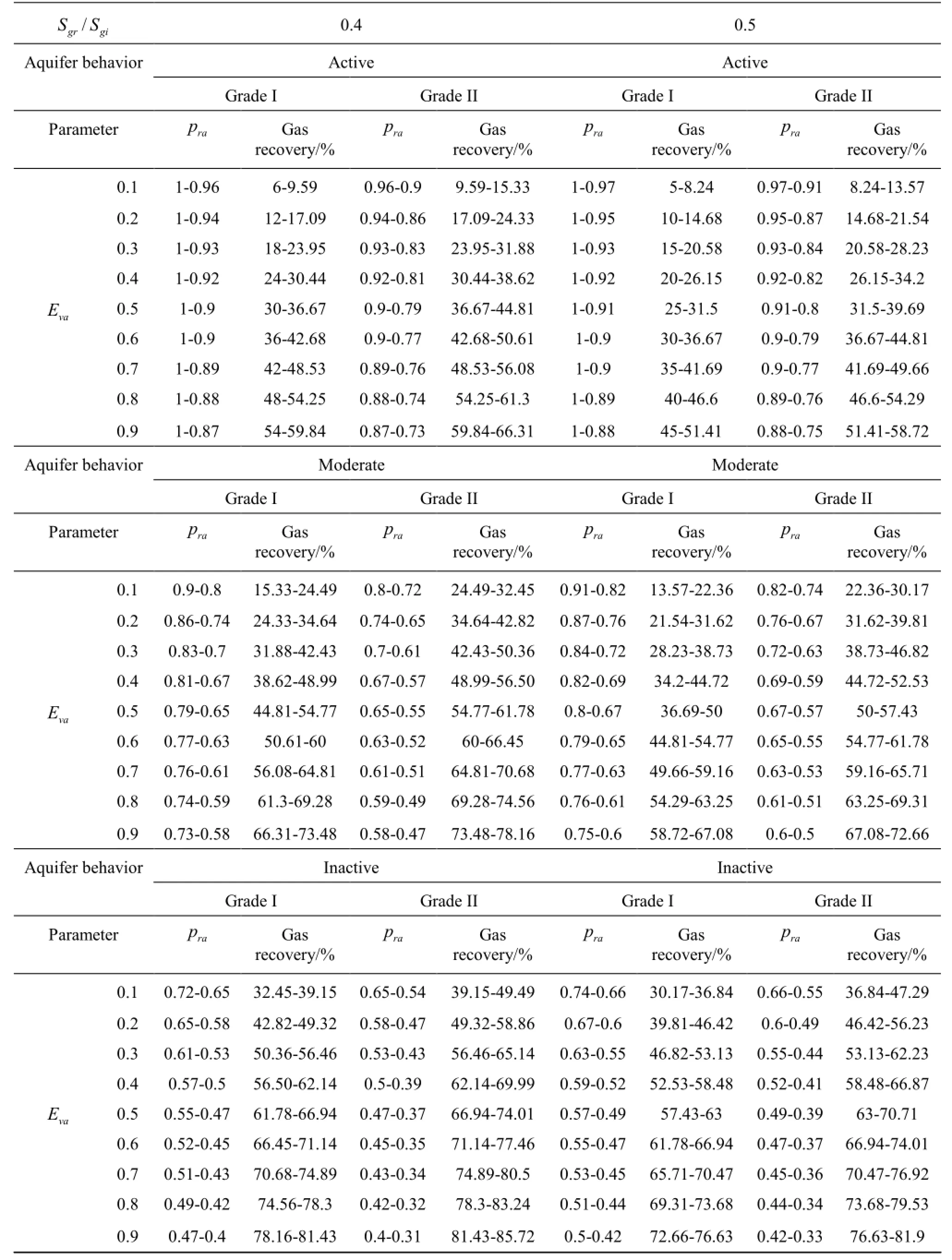
Table 4 Evaluation table

Based on the analysis of above three types of rocks-cemented sandstones， uncemented sandstones and carbonate rocks-it is shown that the reasonable ratio of Sgr/Sgiof the reservoir rocks should range from 0.1 to 0.6 to cover different rocks.

According to statistical results， Nind （1989） suggested that under the abandonment condition， the areal sweep efficiency Eaaranges from 0.6 to 0.95 and the vertical sweep efficiency Ezaranges from 0.6 to 0.9 when the condensate gas reservoirs are abandoned. Thus， the volumetric sweep efficiency of condensate gas reservoirs should be from 0.36 to 0.855. To cover more troublesome reservoirs or formations， e.g.，the reservoirs with fractures， the range of the volumetric sweep efficiency in this paper is chosen to be from 0.1 to 0.9.

3.3Recovery evaluation table and demarcation charts For a specific water-drive gas reservoir， as shown in Fig.2， the extension of the field normalized p/z curve will intersect the normalized end-point line if they are plotted on the same chart. The intersection represents the reservoir performance under the abandonment condition， which is also the only correct point on the normalized end-point line for a specific gas reservoir. It is called the solution point of the gas recovery in our research.

The volumetric sweep efficiency keeps increasing during the exploitation process. When the reservoir is abandoned， the volumetric sweep efficiency is defined as the ultimate volumetric sweep efficiency Eva. According to Fig.2， it is clear that the corresponding normalized p/z of the solution point is the normalized abandonment pa/zawith a certain value ofEvaand the corresponding value of the horizontal coordinate of the solution point is just that of the ultimate gas recovery of the water-drive gas reservoir.

3.3.1Evaluation table

The values of the solution points of different theoretical curves with a certain Evaobtained from the simultaneous solution of Eq.（5） and Eq.（10） are listed in Table 4 （under the condition of Sgr/Sgi=0.4and Sgr/Sgi=0.5， details refer to Yang［18］）， which is called the evaluation table， according to which， the range of the gas recovery at different activity levels of the aquifer behavior can be determined.

3.3.2Evaluation curves

If we plot the normalized end-point lines on Fig.1 with different Evaand Sgr/Sgi， then the recovery evaluation curves with different aquifer behaviors can be obtained as shown in Figs.3， 4. If we put the values of prand Rgof the gas reservoir on Fig.4， for example，the extension of the trend line ofprvs.Rgwill intersect the normalized end-point line. The activity level of the aquifer behavior can be determined according to the area enclosed by the prvs.Rgcurve and the aquifer behavior classification horizontal and vertical coordinates. In addition， the corresponding value of the normalized p/z under the abandonment condition， i.e.， the normalized abandonment pa/zacan be converted into the abandonment pressure when piis given. Thus it can be used to evaluate the ultimate gas recovery for water-drive gas reservoirs in a simple manner whenEvaand Sgr/Sgiare given. The recovery evaluation curves for water-drive gas reservoirs are shown in Figs.3， 4 （the charts whenEva= 0.8 with Sgr/Sgi=0.1and Sgr/Sgi=0.2， respectively）.

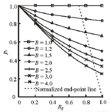
Fig.3 Recovery evaluation curves with Eva=0.8，Sgr/Sgi=0.1

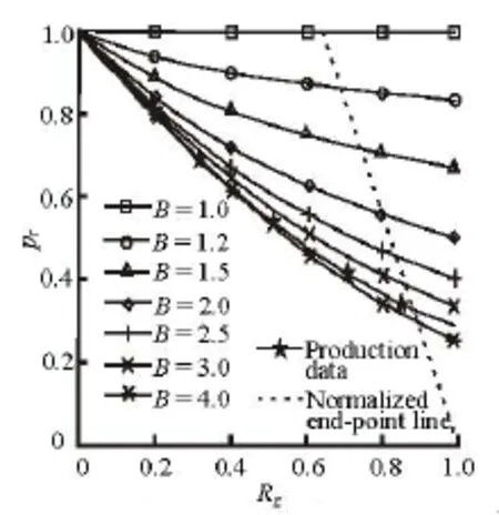
Fig.4 Recovery evaluation curves with Eva=0.8，Sgr/Sgi=0.1

3.3.3Demarcation charts

According to Eq.（5） and Eq.（10）， the relationship between Sgr/Sgiand Rg（Sgr/Sgivs.Rgplot） at different activity levels of the aquifer behavior （differentB） with a certain Evacan be obtained. A groupof the demarcation charts are shown in Figs.5-13. When Sgr/Sgiis given， the gas recovery range can be demarcated by plotting a vertical line regarding the value ofSgr/Sgion the demarcation chart with a certainEva. The intersections of the vertical line and the curves of the chart are the solution points of the ultimate gas recovery. The corresponding vertical coordinate values of adjacent solution points are the limits of the gas recovery for the water-drive gas reservoir with the corresponding aquifer behavior.

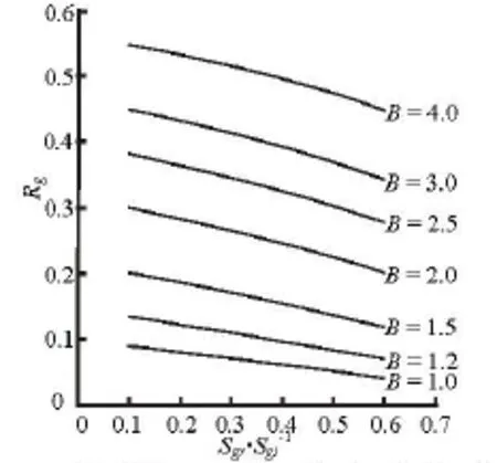
Fig.5 Demarcation chart with Eva=0.1

Fig.6 Demarcation chart with Eva=0.2

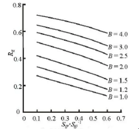
Fig.7 Demarcation chart with Eva=0.3

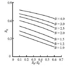
Fig.8 Demarcation chart with Eva=0.4

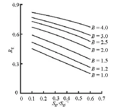
Fig.9 Demarcation chart with Eva=0.5

Fig.10 Demarcation chart with Eva=0.6

4. Case study

4.1Case 1： H3c gas reservoir of Tianwaitian field

The H3c gas reservoir of the Tianwaitian field enjoys good reservoir properties and good connectivity and is a gas reservoir with bottom water. This gas field covers 1.49 km2area with pore volume of 282× 104m3and geological reserve of 3.82×108m3. The specific gravity of the natural gas is 0.61， and the initial formation pressure and temperature are 25.75 MPaand 118.1oC， respectively. According to the experimental measurements， the porosity varies from 2.12% to 20.4%， with an average of 14.499%. The permeability ranges from 1.76 mD to 175 mD， with an average of 43.59 mD.

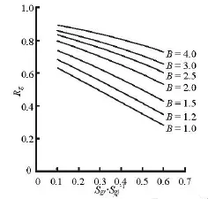
Fig.11 Demarcation chart with Eva=0.7

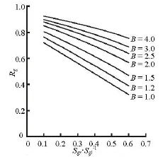
Fig.12 Demarcation chart with Eva=0.8

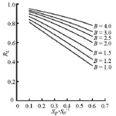
Fig.13 Demarcation chart with Eva=0.9

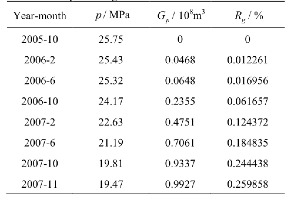
Table 5 The calculation results of the degree of reserve recovery of H3c gas reservoir

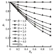
Fig.14 The field normalized p/zcurve of H3c gas reservoir

First， the activity level of the aquifer behavior of the H3c gas reservoir can be determined. According to the values of prand Rgcalculated by the production data （listed in Table 5）， the field normalized p/z curve can be plotted as in Fig.14. From the figure， although there is only a production well in the H3c gas reservoir， the average gas production rate is as high as 14% to 16%. Therefore， the pressure drops rapidly. The field normalized p/zcurve approximately traces one of the curves proposed by Zhang and Li［16］where Bis between 1.5 and 2. According to Fig.14， the water influx coefficient can be estimated as B=1.86. Thus， it is clear that this is a water-drive gas reservoir with the level of moderate grade I of the aquifer behavior. Second， if the corresponding value ofEvain Eq.（10） represents the ultimate volumetric sweep efficiency， the corresponding values of the horizontal and vertical coordinates of the solution point， respectively，represent the ultimate gas recovery and the normalized p/z value under the abandonment condition. Thus it can be used to evaluate the ultimate gas recovery of water-drive gas reservoirs. The water influx is determined by the method proposed by Fetkovich （1971）（listed in Table 6）. By studying the relationship between the residual gas saturation and the original gas saturation of the H3c gas reservoir， it can be found that Swi=0.304，Sgi=0.696and Sgr=0.3205， then Sgr/Sgi=0.4605and Ev=0.338in February 2009（listed in Table 7） based on the formula Ev=（We-WpBw）/Vp（1-Swi-Sgr）proposed by Stoian （1966）. It is assumed here thatBw=1.0. Since there is still a small amount of gas produced after February 2009，Evais chosen in the range from 0.35 to 0.4 as a conjecture. Finally， according to the evaluation table （Table 4）， the gas recovery range of the H3cgas reservoir is from 40.362% to 43.478%.

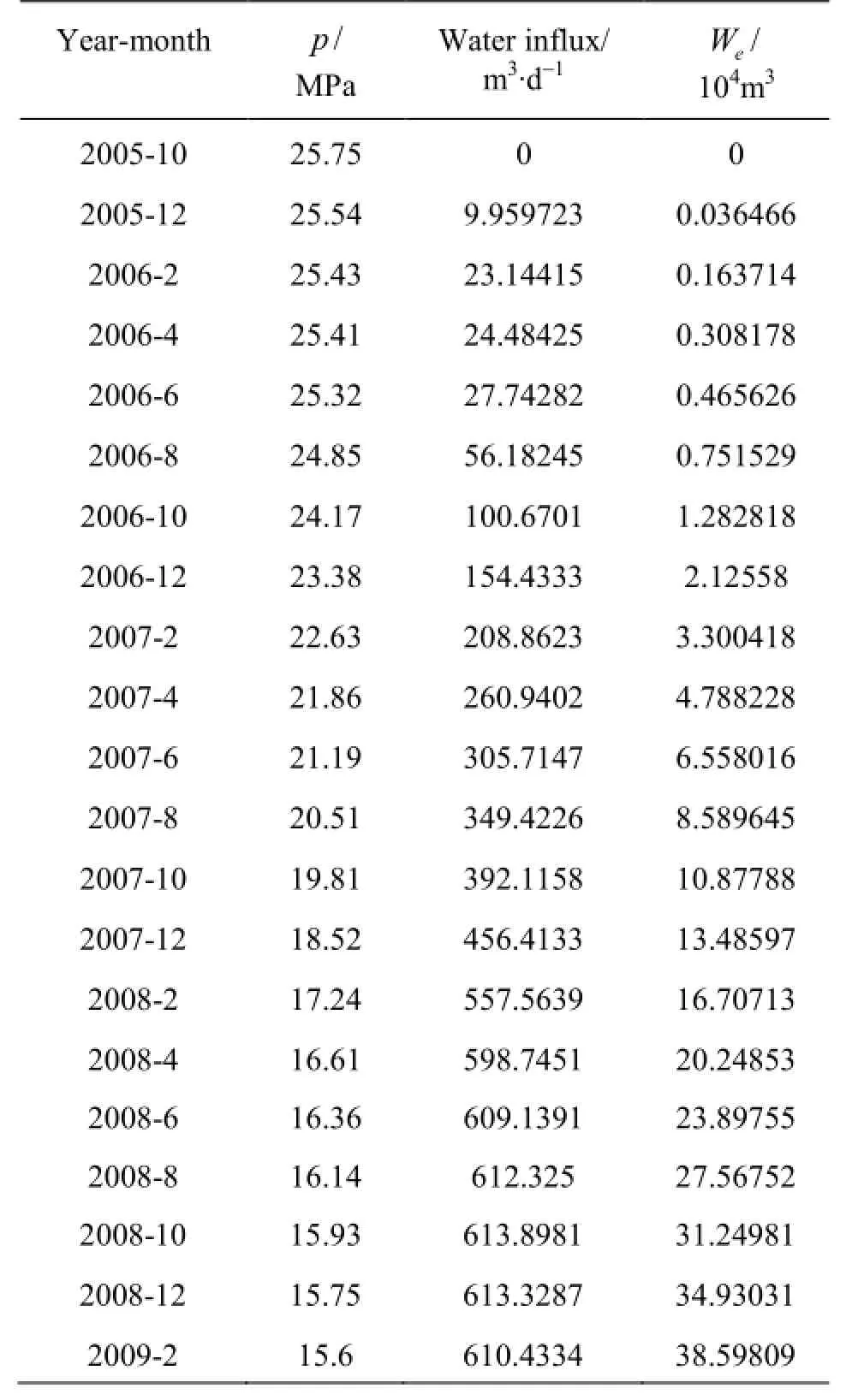
Table 6 The calculation results of water influx of H3c gas reservoir

4.2Case 2： P1 gas reservoir of Pinghu field

This gas field covers 5.22 km2area with pore volume of 1.624×107m3and geological reserve of 2.644×109m3. The specific gravity of the gas is 0.62，and the initial formation pressure is 28.33 MPa and the mid-depth temperature is 118.85oC. Based on the experimental measurements on cores properties， the average porosity and permeability are 19.627% and 185.09 mD， respectively.

First of all， it is necessary to determine the activity level of the aquifer behavior of the P1 gas reservoir. Based on the production data （listed in Table 8），

Table 7 The calculation results of volumetric sweep efficiency of H3c gas reservoir

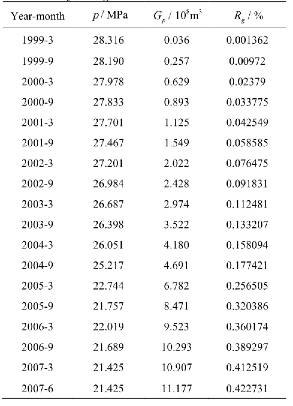
Table 8 The calculation results of the degree of reserve recovery of P1 gas reservoir

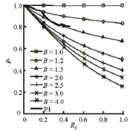
Fig.15 The field normalized p/z curve of P1 gas reservoir

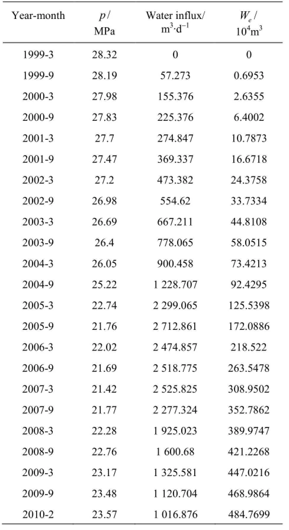
Table 9 The calculation results of water influx of P1 gas reservoir

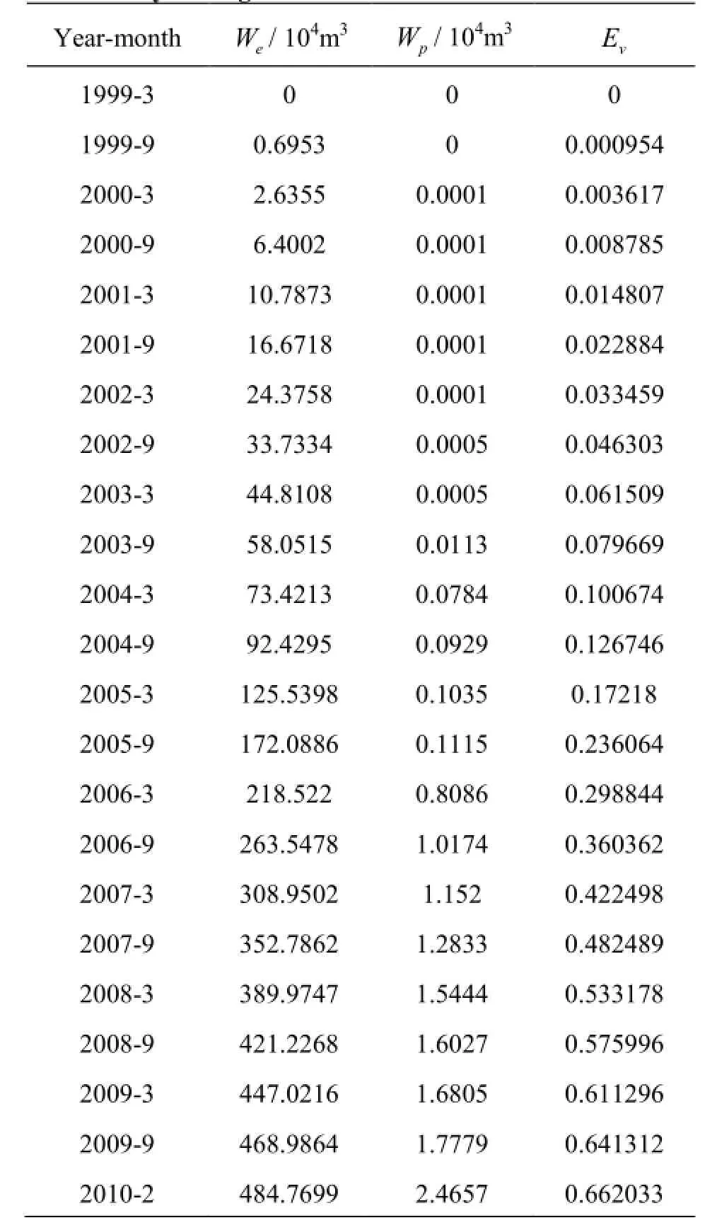
Table 10 The calculation results of volumetric sweep efficiency of P1 gas reservoir

which are used to determine the values of prand Rg，the field normalized p/z curve can be plotted as in Fig.15. Since there is only one production well initially and the gas production rate is less than 5% in the early phase， the pressure declines slowly. After the gas reservoir opens additional production wells， the pressure of the P1 gas reservoir declines more quickly. Finally， the P1 gas reservoir is flooded， and the pressure declines slowly and then is followed by a slight increase. The field normalized p/z curve is approximately consistent with one of the curves proposed by Zhang and Li［16］when the P1 gas reservoir is in the stable production. Based on the late period part of the curve， the water influx coefficient can be obtained B =1.425. According to the classification of the activity level of the aquifer behavior， it can be concluded that this is a water-drive reservoir in the level of active grade II of the aquifer behavior. Second， if the corresponding value of Evain Eq.（10） represents the ultimate volumetric sweep efficiency， the corresponding values of the horizontal and vertical coordinates are under the solution condition. The calculation results ofthe water influx are listed in Table 9 according to the formulae proposed by Fetkovich （1971）. According to the laboratory study，Sgr=0.3246and Sgi=0.773，thenSgr/Sgi=0.4199. Thus it is determined that Ev=0.662in February 2010 （listed in Table 10）based on the formulaEv=（We-WpBw）/Vp（1-Swi-Sgr）proposed by Stoian （1966）. Because there are still a few gas produced after February 2010，Evais chosen in the range from 0.70 to 0.75 as a guess. Finally， according to the evaluation table （Table 4），the range of the ultimate gas recovery is from 55.502% to 58.111%.

5. Conclusions

（1） A new classification method is developed for determining the levels of the aquifer behavior based on the production performance， with which the waterdrive gas reservoirs are classified into six types： the influx reservoirs in the levels of active grade I（1＜ B＜1.2）and grade II （1.2＜B＜1.5）， moderate grade I（1.5＜B＜2）and grade II （2＜B＜2.5）and inactive grade I（2.5＜B＜3）and grade II （3＜B＜4）.

（2） The recovery of water-drive gas reservoirs can be estimated or demarcated based on the evaluation table or the demarcation charts proposed in this paper. In this manner， the gas recovery for water-drive gas reservoirs can be determined if values ofEvaand Sgr/Sgiare given.

（3） According to the case studies， the field normalized p/zcurves approximately trace the curves proposed by Zhang et al..

Acknowledgement

The authors acknowledge the contributions of Mrs. Xiao Qian-yin who guided the translation.

References

［1］EL-AHMADY M. H.， WATTENBARGE R. A. Overestimation of original gas in place in water-drive gas reservoirs due to a misleading linear p/z plot［C］. Canadian International Petroleum Conference. Calgary， Canada， 2001.

［2］GLEGOLA M. A.， DITMAR P. and HANEA R. G. et al. Gravimetric monitoring of water influx into a gas reservoir： A numerical study based on the ensemble kalman filter［J］. SPE Journal， 2012， 17（1）： 163-176.

［3］HU J. K.， LI X. P. and YANG H. L. A new method for determining original gas in place and cumulative water influx in water drive gas reservoirs［C］. International Conference on Computational and Information Sciences. Shiyang， China， 2013.

［4］PUJIASTUTI D.， ARIADJI T. A recovery factor correlation for a bottom water drive gas reservoirs［C］. Indonesian Petroleum Association Twenty-Eighth Annual Convention. Jakarta， Indonesia， 2002.

［5］SHENG Ru-yan. Experimental study on residual gas saturation of water-flooded sandstone reservoirs［J］. Journal of Oil and Gas Technology， 2010， 32（4）： 105-107（in Chinese）.

［6］PAPAY J. A correlation method for determination of residual non-wetting saturation［J］. Erdol Erdgas Kohle，2004， 120（12）： 162-165.

［7］HOLTZ M. H. Residual gas saturation to aquifer influx：A calculation method for 3-D computer reservoir model construction［C］. SPE Gas Technology Symposium. Alberta， Canada， 2002.

［8］MULYADI H.， AMIN R. and KENNAIRD T. et al. Measurement of residual gas saturation in water-driven gas reservoirs： Comparison of various core analysis techniques［C］. International Oil and Gas Conference and Exhibition. Beijing， China， 2000.

［9］LI Jiu-di， HU Ke. Experimental study of residual gas saturation at DH gas reservoir［J］. Journal of Southwest Petroleum University， 2014， 36（1）： 107-112（in Chinese）.

［10］SUZANNE K.， HAMON G. and BILLIOTTE J. et al. Experimental relationships between residual gas saturation and initial gas saturation in heterogeneous sandstone reservoirs［C］. SPE Annual Technical Conference and Exhibition. Denver， America， 2003.

［11］LE D. H.， HOANG H. N. and MAHADEVAN J. Gas recovery from tight sands： Impact of capillarity［J］. SPE Journal， 2012， 17（4）： 981-991.

［12］KHAN C.， AMIN R. and MADDEN G. Economic modelling of CO2injection for enhanced gas recovery and storage： A reservoir simulation study of operational parameters［J］. Energy and Environment Research， 2012，2（2）： 65-82.

［13］HUGHES T. J.， HONARI A. and GRAHAM B. F. et al. CO2sequestration for enhanced gas recovery： New measurements of supercritical CO2-CH4dispersion in porous media and a review of recent research［J］. International Journal of Greenhouse Gas Control，2012， 9： 457-468.

［14］LI Zhong-xing， HAO Yu-hong. The correction of volume method for calculating gas reservoir recovery and recoverable reserves［J］. Natural Gas Industry， 2001，21（2）： 71-75（in Chinese）.

［15］WU Yi-lu， LI Xiao-ping and LI Hai-tao. The prediction method of recovery for natural gas condensate reservoir of depletion development［J］. Journal of Southwest Petroleum University， 2004， 26（4）： 38-40（in Chinese）.

［16］ZHANG Lun-you， LI Jiang. Curve-fitting method of calculating dynamic reserve of water drive gas reservoir［J］. Natural Gas Industry， 1998， 18（2）： 26-29（in Chinese）.

［17］LI Chuan-liang. Fundamentals of reservoir engineering［M］. Beijing， China： Petroleum Industry Press，2005（in Chinese）.

［18］YANG Hai. Study of the recovery of T water-drive gas reservoir［D］. Master Thesis， Chengdu， China： South-West Petroleum University， 2012（in Chinese）.

（January 28， 2014， Revised June 9， 2014）

* Project supported by the National Natural Science Foun-dation of China （Grant Nos. 41274114， 51274169）， the National Science and Technology Major Project of China （Grant No. 2011ZX05045）.

Biography： LI Min （1962-）， Male， Ph. D.， Professor