Numerical analyses of pressure fluctuations induced by interblade vortices in a model Francis turbine*

ZUO Zhi-gang （左志钢）， LIU Shu-hong （刘树红）， LIU De-min （刘德民）， QIN Da-qing （覃大清），Wu Yu-lin （吴玉林）

1. Department of Thermal Engineering， State Key Laboratory of Hydro Science and Engineering， Tsinghua University， Beijing 100084， China， E-mail：zhigang200@tsinghua.edu.cn

2. Research and Test Center， Dongfang Electric Machinery Co. Ltd， Deyang 618000， China

3. State Key Laboratory of Hydro-power Equipment， Haerbin 150001， China

Numerical analyses of pressure fluctuations induced by interblade vortices in a model Francis turbine*

ZUO Zhi-gang （左志钢）1， LIU Shu-hong （刘树红）1， LIU De-min （刘德民）2， QIN Da-qing （覃大清）3，Wu Yu-lin （吴玉林）1

1. Department of Thermal Engineering， State Key Laboratory of Hydro Science and Engineering， Tsinghua University， Beijing 100084， China， E-mail：zhigang200@tsinghua.edu.cn

2. Research and Test Center， Dongfang Electric Machinery Co. Ltd， Deyang 618000， China

3. State Key Laboratory of Hydro-power Equipment， Haerbin 150001， China

Interblade vortices can greatly influence the stable operations of Francis turbines. As visible interblade vortices are essentially cavitating flows， i.e.， the ones to cause interblade vortex cavitations， an unsteady simulation with a method using the RNG k-εturbulence model and the Zwart-Gerber-Belamri （ZGB） cavitation model is carried out to predict the pressure fluctuations induced. Modifications of the turbulence viscosity are made to improve the resolutions. The interblade vortices of two different appearances are observed from the numerical results， namely， the columnar and streamwise vortices， as is consistent with the experimental results. The pressure fluctuations of different frequencies are found to be induced by the interblade vortices on incipient and developed interblade vortex lines， respectively， on the Hill diagram of the model runner's parameters. From the centrifugal Rayleigh instability criterion， it follows that the columnar interblade vortices are stable and the streamwise interblade vortices are unstable in the model Francis turbine.

interblade vortices， pressure fluctuations， Francis turbine， cavitation， Rayleigh instability

Introduction

It is known that the existence of interblade vortices can induce instabilities in the operations of Francis turbines. For instance， severe vertical vibrations （over 200 µm） in the guide bearings， as well as major horizontal cracks （～1m）in the draft tube cones， were observed on Units Nos. 13 and 14 of Pakistan's Tarbela Power Station at high head after about 6 months of their commissioning. These issues， pointed out by the manufacturer， DBS-Escher Wyss in Canada，are associated with interblade vortices at high head in the units［1］. Through experimental analyses of the model and prototype runners， Alstom had observed cracks in the runners of two Brazilian hydroelectric power stations as induced by the interblade vortices at low head［1］. The source of the extensive noise in the rehabilitated turbines in the Gongzui Power Station was verified to be the interblade vortices under low load operating conditions［2］.

Due to the strong influence of the interblade vortices on the hydraulic instability of the runner， it is desirable to study the characteristics of the vortical flows and the induced pressure fluctuations. Experimental studies so far focused on the identifications of these vortices. Grindoz made observations regarding the visible interblade vortices in a model Francis turbine［3］. A series of experimental studies of the model runner for the Three Gorges power station reveals that the interblade vortices occur from the runner inlet under high head working conditions［4，5］. It is indicated that the existence of the vortices could induce alternating loads on the runner blades， resulting in fatigue damages. Most of the numerical researches were carried outthrough single-phase flow simulations， but no conclusive frequency characteristics of the pressure fluctuations induced by the interblade vortices were obtained［6-8］.

It is shown that the visible vortices in the model tests' interblade flow channels are cavitating flows，i.e.， interblade vortex cavitation （Fig.1）［9］. Thus it is clear that single-phase flow simulations are not adequate to model the complex process of this phenomenon. Kurosawa built a numerical model to predict the major characteristics， including the occurrence of the interblade vortices， by solving the Reynolds averaged Navier-Stokes （RANS） equations， combined with the Reynolds Stress model and the volume of fluid （VOF）method［10］. Reasonable agreements were achieved between numerical and experimental results.

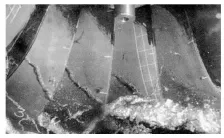
Fig.1 Interblade （cavitating） vortices in a Francis turbine runner

Since the pressure fluctuations are closely related to the behavior of the vortical flows， it is important to study the characteristics of the vortices. Analyses of the stability of the vortex ropes in Francis turbines were made to account the physical origin of severe low-frequency pressure fluctuations in their draft tubes［11，12］.

In this paper， in order to provide guidelines for safe operations with respect to interblade vortices，analyses are carried out for the stability of the vortices of different appearances in a Francis model turbine，based on unsteady simulation results from the RNG k-εturbulence model and the Zwart-Gerber-Belamri（ZGB） cavitation model. Modifications on the turbulence viscosity are made for better resolutions.

1. Numerical methods

1.1Cavitation simulation

The simulations of cavitating flows can be performed by taking the vapor/liquid mixture as a multiphase single fluid， with variable densities. No slip exists between the two phases in this mixture model. Therefore， only one set of momentum equations are needed to describe the pressure and the velocities of the mixture［13］. Various forms of cavitation models were proposed to account for the mass transfers between the two phases in the additional continuity equation of the vapor phase， e.g.， the cavitation model by Merkle［14］， Kunz［15，16］， Singhal［17］， Senocak and Shyy［18］. The so-called ZGB cavitation model is applied in this study， which considers the variation of the volume fractions of the cavitation nuclei， and evaluates the rate of mass transfer through a simplified Rayleigh-Plesset equation［19］. The continuity equation for the vapor phase and the expressions of the two source terms，Reand Rc， of the model are as follows：

wheresgnin sgn（pv-p）is the sign function，αv，ρvrepresent the volume fraction and the density of the vapor， respectively，pvdenotes the vapor pressure，αnucis the nucleation site volume fraction，RBis interpreted as the radius of the nucleation site，Fvap，Fconare two empirical calibration coefficients. In our calculations，Fvap=80，Fcon=0.01， and the default values for other parameters are specified.

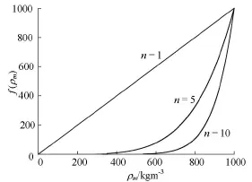
Fig.2f（ρm）-ρm

As stated above， the RANS equations in this study are solved by adapting the RNG k-εturbulence model and the ZGB cavitation model［20］. It is indicated that the turbulence viscosity is usually overestimated in the cavitation simulations due to the use of the mixture model， and modifications of the temporal and spatial discretization schemes alone are not enough to offset this effect［21］. Based on the study ofCoutier-Delgosha［22，23］， a modification of the turbulence viscosity µtfrom the Boussinesq eddy viscosity assumption is adopted in this study，

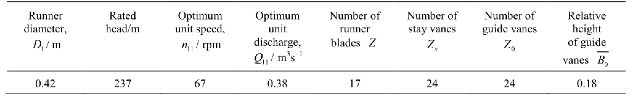
Table 1 Parameters of the model Francis turbine

wherek，εare the turbulent kinetic energy and its dissipation rate， respectively，ρv，ρl， and ρmrepresent the density of the vapor， the liquid， and the mixture， respectively， the functionf（ρm）is introduced to consider the influence of the variations in density on the turbulence viscosity. As shown in Fig.2， the value of the exponentncontrols the shape of f（ρm）against ρmn=10is chosen in this study as suggested by the references mentioned above.

1.2Model Francis turbine

The numerical studies are conducted with a model Francis turbine， the parameters of which are listed in Table 1. The computational domain is shown in Fig.3.

Fig.3 Computational domain

The model gives a 94.54% level of peak efficiency. The performance characteristics determined by model tests under an experimental head of 30 m are shown in Fig.4， where Q11is the discharge，n11is the rotating speed. The experiments are performed on the Test Rig II of Harbin Electric Corporation as a part of the acceptance test of the unit. The systematic uncertainty on the efficiency measurement of the test rig is less than ±0.25%.

Fig.4 Hill diagram for parameters

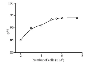
Fig.5 Verification of grid independence

1.3Computational details

The model's mesh system is composed of unstructured grids fpr the spiral case， the stay vanes and the runner， and structured grids for the guide vanes， the draft tube， and the inlet pipe. The commercial software package ICEM is used for the mesh discretization. The local refinements to the boundary layer in the runner are applied in order to ensure the values of y+to be compatible with the chosen turbulence model. The grid independence is verified with respect to the runner efficiency， with the total number of grid cells varying from 2×106to 8×106， as shown in Fig.5. It can be seen that the degree of the computational precision is satisfactory when the number of cells is greater than 6×106. A mesh with about 7.6×106cells in total is chosen for the simulations. The numbers of nodes and cells in each part are shown in Table 2.

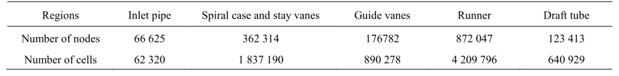
Table 2 Numbers of cells and nodes of each subdomain

Table 3 Comparison of parameters between cavitation calculations and experiments

The time step for the unsteady simulations is set as 2.17×10-4s （when the runner rotates by 1o）. A second-order upwind scheme is used for the discretization of the convective terms， and a second-order centered scheme is used for the source terms. The total pressure， the initial values of the turbulent kinetic energy and the turbulent dissipation rates are set on the inlet boundary， while the static pressure is set as the outlet boundary condition.

2. Cavitation calculations and predictions of vortex lines

The numerical method is validated through the unsteady flow calculations with different cavitation numbers at the operating Point A （n11=58.86，Q11= 0.43，a=0.018m）， as well as the predictions of the incipient and developed interblade vortex lines with steady flow calculations， as shown in Fig.4.

Fig.6 Pressure monitoring points

For the cavitation calculations， the cavitation number is defined in terms of the static pressure at the draft tube outlet

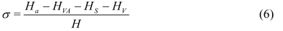
where HVA=pVA/ρgis the pressure head in the low pressure tank，Ha=pa/ρgis the atmospheric pressure head， andHSis the suction head of the turbine with respect to the centerline of the guide vanes. HV=pV/ρgis the saturated vapor pressure head at the experimental temperature.

As shown in Table 3， the numerical predicted efficiencyηand powerPagree well with the experimental observations. In order to evaluate the calculated unsteady pressure fluctuations against the experiments， the pressure monitoring Points G1， G2 and D1，D2， D3， D4 are chosen in the vaneless space and the draft tube， as shown in Fig.6. As seen in Table 4， minute differences can be observed between the numerical and the experimental results of the relative amplitude （ΔH/H， where ΔHis the characteristic amplitude of the pressure fluctuations， with a 97% probability［24］）， and the dominant frequency of the pressure fluctuations at the monitoring points.

Furthermore， the predictions of the incipient and developed interblade vortex lines are made. In order to determine the incipience of the interblade vortices in the model acceptance tests， we identify the visible vortices in two or three interblade flow channels simultaneously. When the visible vortices occur in all interblade flow channels， we say that the interblade vortices are developed. The lines connecting the operating points on the Hill diagram in the parameters（Q11-n11）with the incipient and initial occurrence of the developed interblade vortices are called the incipient interblade vortex line， and they and the developed interblade vortex lines are ， respectively， shown in Fig.4. In order to predict the two interblade vortex lines， it is essential to evaluate the compatibility of various vortex identification methods in our simulation cases. A number of vortex identification methods/criteria were proposed［25］， including the vorticity criterion， theQ criterion， the swirling strength criterion，and the helicity criterion. By comparing the isosurfaces of the four quantities at corresponding operating points with n11=59r/min， and n11=72.5r/min，along the incipient and developed interblade vortex lines， respectively， it can be concluded that the vorticity criterion is most suitable for distinguishing the vortices. N inen11valuesare cho sen， each u nder 3-6 operatingconditionsforsteadycavitationcalculations，and the incipient and developed interblade vortex lines are asymptotically derived based on the vorticity criterion. As shown in Fig.7， good agreements are achieved by using the prescribed cavitation calculations. It can be seen below that the inflection points on both lines are successfully predicted.

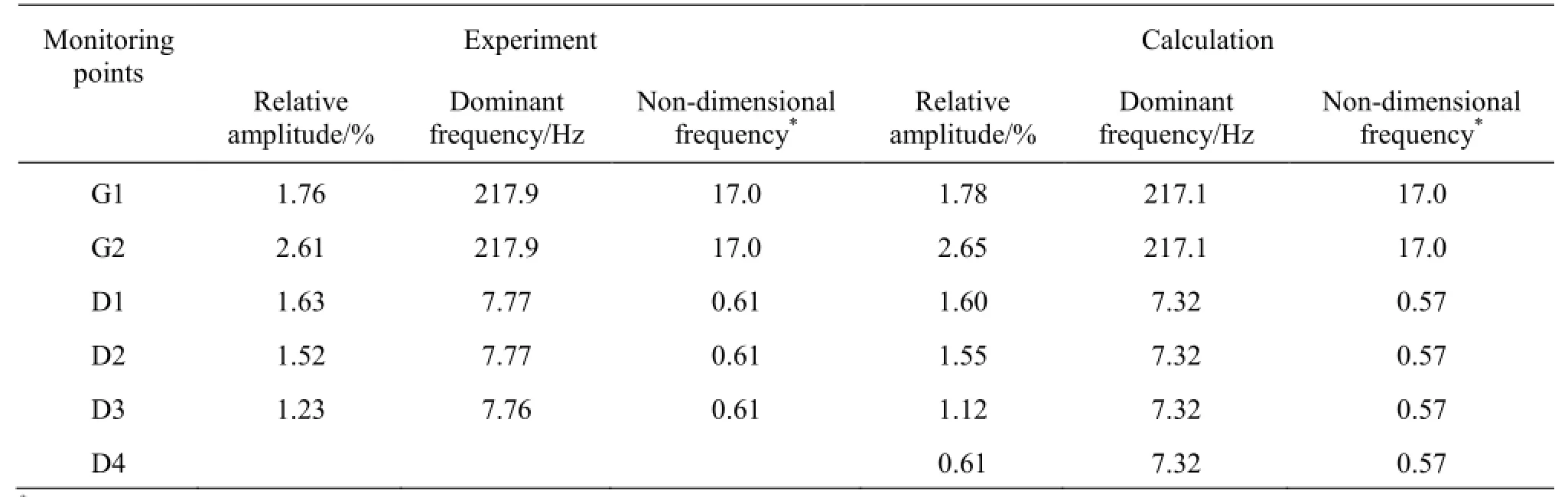
Table 4 Pressure fluctuations in the turbine

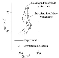
Fig.7 Predictions of the incipient and the developed interblade vortex lines

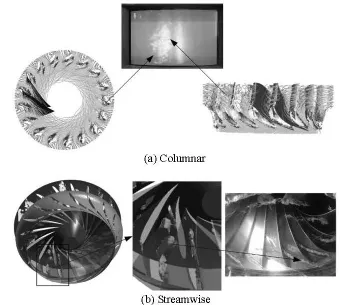
Fig.8 Appearances of interblade vortices

Fig.9 Monitoring points on runner blades

3. Hydraulic stability analysis of interblade vortices

As shown in Fig.8， the two main appearances of the interblade vortices， namely， the columnar vortices near the runner inlet and the streamwise vortices further inside the interblade channels， are recognized in this study's simulation results of the turbine unit，which agree well with the experimental observations. In order to study the unsteady characteristics of the interblade vortices， we investigate two operating points， B （a =0.010m，=58.7r/min，Q=0.235m3/s）11and C （a =0.008m，n11=58.7r/min，Q11= 0.190m3/s） on the incipient interblade vortex line and the developed interblade vortex line （Fig.4）. 18 monitoring points are located on the pressure side and the suction side of the runner blades to study the development of the interblade vortices， as shown in Fig.9. They are arranged in the direction of the flows near the crown （Pc1-Pc3， Sc1-Sc3）， in the middle （Pm1-Pm3， Sm1-Sm3）， and near the band （Pb1-Pb3， Sb1-Sb3）， respectively.

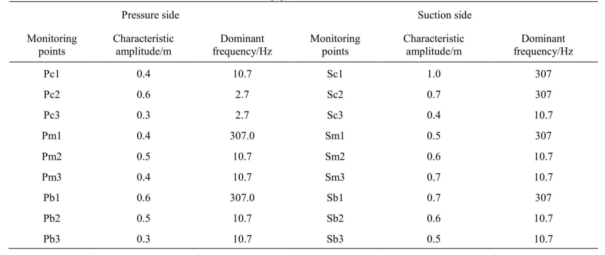
Table 5 Pressure fluctuations on turbine runner blades （B）

Table 6 Pressure fluctuations on turbine runner blades （C）

Table 5 shows the pressure fluctuations at the prescribed monitoring points on the turbine runner blades at the operating Point B. The pressure fluctuation components with three frequencies are observed，307 Hz （the guide vane passing frequency）， 2.7 Hz（the frequency of the pressure fluctuation induced by the draft tube vortex rope）， and 10.7 Hz， which is believed to be the frequency of the pressure fluctuations induced by the interblade vortices， at almost all monitoring points. Comparing with Table 4， considerable differences in the pressure fluctuation frequencies exist between the stationary and rotating parts of the unit. The guide vane passing frequency Z0fnis a main component in the runner， while the runner blade passing frequencyZfnis a main component in the guide v anes.Si ncethe inte rbladevorti ces occuron the suctionsideofthebladesunderthisworkingcondition， higher amplitudes of the pressure fluctuations are observed there. The pressure fluctuations at the operating Point C have smaller amplitudes， and a slightly different frequency for the pressure fluctuations induced by the interblade vortices （12.8 Hz）， as shown in Table 6. In both cases， higher amplitudes of the pressure fluctuations are observed near the runner crown and band， instead of the middle of the runner. An attempt is made to qualitatively account for this phenomenon by analyzing the stability of the vortices with different appearances.

For inviscid fluids， Rayleigh provided an argument to determine the stability of a revolving flow with respect to axisymmetric disturbances. As shown in Fig.10， consider the interchange of the fluid in two rings of radii r1and r2. Following the conservation of the angular momentum， it is shown that in the caseof r2＞r1， the condition for the flow instability is d（Ωr2）2/dr＜0somewhere， in whichΩis the angular velocity［26，27］. Since the vortices have strong circumferential components that resemble the revolving flows， the prescribed centrifugal Rayleigh instability criterion can be roughly applied in a preliminary analysis.

Fig.10 Rayleigh instability criterion

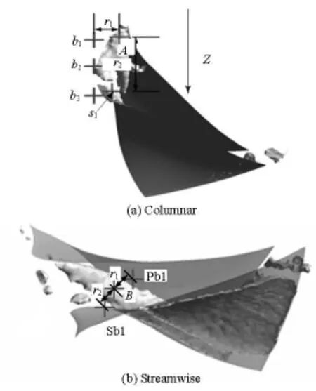
Fig.11 Rayleigh stability analysis of interblade vortices

As shown in Fig.11， several pairs of monitoring points are selected for analysis （b1and s1around the columnar vortex center A， Sb1 and Pb1 around the streamwise vortex center B， etc.）. In the cases studied，theΩr2values vary as time evolved. As an example，Fig.12 shows the time series ofΩr2at the points Sb1 and Pb1. The time averaging values are selected for analysis， and it is found thatd（Ωr2）2/dr＜0is the condition fpr the occurrence of the streamwise interblade vortices， whiled（Ωr2）2/dr＞0is the condition for the occurrence of the columnar interblade vortices（see Table 7 for example）. This indicates that in the model Francis turbine studied in this paper the streamwise interblade vortices are unstable， while the columnar interblade vortices are stable. This is in accordance with the phenomenon that the pressure fluctuations at the middle of the runner blades are weaker， while those near the runner band are stronger.

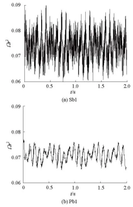
Fig.12 Time series of Ωr2at monitoring points

4. Conclusions

In order to predict the pressure fluctuations induced by interblade vortices， a method of cavitation calculations is proposed， which consists of solving the RANS equations with the RNG k-εturbulence model and the ZGB cavitation model. Turbulence viscosity modifications are made to compensate its overestimation in the cavitation area.

The method is validated by successful predictions of the pressure fluctuations of the cavitating flows in the turbine runner， and of the incipient and developed interblade vortex lines， where the vorticity criterion is chosen for identifying the vortices. The incipient and developed interblade vortex lines are determined by observing the occurrence of the interblade vortices from the steady flow calculation results. Operating points where the vortices occur simultaneously in two or three inter blade flow channels form the incipient interblade vortex line， and when visible vortices occur in all inter blade flow channels， we say that the interblade vortices are developed.

Interblade vortices of two appearances are observed in the numerical results， namely， the columnar and streamwise vortices， which agree with the experimental results. The evaluations of the pressure fluctuati onsind uced by theinterb lade vortices arethen madeonthemonitoringpointslocatedonbothsidesof the runner blades at two operating points， on the incipient and developed interblade vortex lines. It is found that the interblade vortices induce pressure fluctuations with different frequencies on the two vortex lines. A preliminary analysis of the stability of the vortices is carried out to explain the phenomena that the pressure fluctuations at the middle of the runner blades are weaker， while the fluctuations near the band are stronger. From the centrifugal Rayleigh instability criterion， it follows that the columnar interblade vortices are stable and the streawise interblade vortices are unstable in the model Francis turbine studied.

Table 7 Comparisons of Ωr2values

Further studies of different turbine runners are needed to investigate the applicability of this instability argument of interblade vortices.

References

［1］HUANG Yuan-fang， LIU Guang-ning and FAN Shiying. Research on prototype hydro-turbine operation［M］， Beijing， China， China Electric Power Press，2010（in Chinese）.

［2］SHI Qing-hua， XU Wei-wei and GONG Li. Noise reduction in a low head Francis turbine caused by runner inter-blade vortices［J］. Dongfang Electrical Machine，2008， （1）： 42-46（in Chinese）.

［3］GRINDOZ B. Lois de similitudes dans les essays de cavitation des turbines Francis［D］. Doctoral Thesis，Lausanne， Switzerland： EPFL， 1991.

［4］PENG Zhong-nian， CHEN Rui and JIANG Xue-yun. Experimental investigation of flow pattern observation and water pressure pulsation performed on the Three Gorges model turbine［J］. Water Resources and Hydropower Engineering， 1999， 30（11）： 8-14（in Chinese）.

［5］CHEN Rui， PENG Zhong-nian. An experimental study on water pressure fluctuation at Francis turbine runner blade outlet［J］. Water Resources and Hydropower Engineering， 1999， 30（11）： 30-32（in Chinese）.

［6］CHEN Jin-xia， LI Guo-wei and LIU Sheng-zhu. The occurrence and the influence of the interblade vortex on the hydraulic turbine instability［J］. Large Electric Machine and Hydraulic Turbine， 2007， （3）： 42-46（in Chinese）.

［7］ZHANG Peng-yuan， ZHU Bao-shan and ZHANG Le-fu. Numerical investigation on pressure fluctuations induced by interblade vortices in a runner of Francis turbine［J］. Large Electric Machine and Hydraulic Turbine， 2009， （6）： 35-39（in Chinese）.

［8］STEIN P.， SICK M. and DOERFLER P. et al. Numerical simulation of the cavitating draft tube vortex in a Francis turbine［C］. IAHR Section Hydraulic Machinery， Equipment， and Cavitation， 23rd Symposium. Yokohama， Japan， 2006.

［9］AVELLAN F. Introduction to cavitation in hydraulic machinery［C］. 6th International Conference on Hydraulic Machinery and Hydrodynamics. Timisoara，Romania， 2004.

［10］KUROSAWA S.， LIM S. M. and ENOMOTO Y. Virtual model test for a Francis turbine［C］. 25th IAHR Symposium on Hydraulic Machinery and Systems. Timisoara， Romania， 2010.

［11］ZHANG R.， CAI Q. and WU J. et al. The physical origin of severe low-frequency pressure fluctuations in giant Francis turbines［J］. Modern Physics Letters B，2005， 19（28-29）： 1527-1530.

［12］WU J.， CHEN S. and WU Y. et al. Characteristics and control of the draft-tube flow in part-load Francis turbine［J］. Journal of Fluids Engineering， 2009， 131（2）. 021101.

［13］SENOCAK I.， SHYY W. A pressure-based method for turbulent cavitating flow computations［J］. Journal of Computational Physics， 2002， 176（2）： 363-383.

［14］MERKLE C.， FENG J. and BUELOW P. Computational modeling of the dynamics of sheet cavitation［C］. Proceeding of Third International Symposium on Cavitation. Grenoble， France， 1998， 307-311.

［15］KUNZ R. F.， BOGER D. A. and CHYCZEWSKI T. S. et al. Multi-phase CFD analysis of natural and ventilated cavitation about submerged bodies［C］. ASME Fluid Engineering Division Summer Meeting，FEDSM99-7364. San Francisco， USA， 1999.

［16］KUNZ R.， BOGER D. and STINEBRING D. A Preconditioned Navier-Stokes method for two-phase flows with application to cavitation prediction［J］. Computers and Fluids， 2000， 29（8）： 849-875.

［17］SINGHAL A. K.， ATHAVALE M. M. and LI H. et al. Mathematical basis and validation of the full cavitation model［J］. Journal of Fluids Engineering， 2002， 124（3）：617-624.

［18］SENOCAK I.， SHYY W. Interfacial dynamics-based modeling of turbulent cavitating flows，model development and steady-state computations［J］. International Journal for Numerical Methods in Fluids， 2004，44（9）： 975-995.

［19］ZWART P.， GERBER A. and BELAMRI T. A twophase flow model for predicting cavitation dynamics［C］. Fifth International Conference on Multiphase Flow. Yokohama， Japan， 2004.

［20］LIU Yan， ZHAO Peng-fei and WANG Qiang et al. URANS computation of cavitating flows around skewed propellers［J］. Journal of Hydrodynamics， 2012，24（3）： 339-346.

［21］COUTIER-DELGOSHA O.， REBOUD J. Numerical simulation of unsteady cavitation flows［J］. InternationalJournal for Numerical Methods in Fluids， 2003，42（5）： 527-548.

［22］COUTIER-DELGOSHA O.， FORTES-PATELLA R. and REBOUD J. Evaluation of the turbulence model influence on the numerical simulations of unsteady cavitation［J］. Journal of Fluids Engineering， 2003， 125（1）：38-45.

［23］COUTIER-DELGOSHA O.， REBOUD J. and ALBANO G. Numerical simulation of the unsteady cavitation behavior of an inducer blade cascade［C］. ASME Proceedings of ASME Fluids Engineering Division Summer Meeting. Boston， Massachusetts， USA， 2000.

［24］Hydraulic turbines， storage pumps and pump-turbines-Model acceptance tests［S］. International Standard IEC 60193， 1999.

［25］HANSEN C. D.， JOHNSON C. R. Visualization Handbook［M］. Burlington， Canada： Butterworth-Heinemann， 2005， 295-309.

［26］RAYLEIGH L. On the dynamics of revolving fluids［J］. Proceedings of the Royal Society of London， Series A，1917， 93（648）： 148-154.

［27］DRAZIN P. G.， REID W. H. Hydrodynamic stability［M］. 2nd Edition， Cambridge， UK： Cambridge university Press， 2004.

（February 6， 2014， Revised March 10， 2014）

* Project supported by the National Natural Science Foundation of China （Grant No. 51476083）， the National Science and Technology Ministry of China （Grant No. 2011BAF03B01）.

Biography： ZUO Zhi-gang （1977-）， Male， Ph. D.