Analysis method on error distributions of in-flight alignment schemes
2015-06-05WENGJunQINYongyuanYANGongminMEIChunbo
WENG Jun, QIN Yong-yuan, YAN Gong-min, MEI Chun-bo
(Department of Automatic Control, Northwestern Polytechnical University, Xi’an 710129, China)
Analysis method on error distributions of in-flight alignment schemes
WENG Jun, QIN Yong-yuan, YAN Gong-min, MEI Chun-bo
(Department of Automatic Control, Northwestern Polytechnical University, Xi’an 710129, China)
When carrier aircrafts have emergency combat tasks, they may quickly take off first, and then do the in-flight alignment. In order to guarantee the inertial navigation system reaching a certain precision index when entering navigation mode after the alignment process, the attitude information at the end of the alignment needs to meet a certain accuracy requirement. The in-flight alignment process normally can be divided into two parts: coarse alignment and precise alignment. The attitude precision at the end of the precise alignment is determined by coarse alignment, inertial measurement unit error, gravity field model error and in-flight maneuver through alignment process, etc. Firstly, a covariance analyzing method is designed and used to get error distributions of two different alignment schemes. Then, Monte-Carlo simulation technique is used to testify the accuracy of error distribution results. Simulation results show that the proposed analysis method is correct, which can provide reference for improving in-flight alignment schemes.
in-flight alignment; error distributions; covariance analysis; Monte-Carlo simulation
In-flight alignment process of carrier aircraft normally can divided into two parts, one is coarse alignment, which can be accomplished using inertial frame alignment algorithm[1-4]; one is precise alignment, which always use INS/GPS integrated scheme, whose integrated mode is“velocity + position”[5-7]. As to fulfill established indexes for alignment task, every error sources affecting in-flight alignment should be analyzed, which means how much influence every potential error can have on the attitude precision at end of alignment process.
Main errors of in-flight alignment are of two different aspects: IMU’s error and external measurements’ error, which all involved in Kalman filtering part in navigation computer. It is obvious to establish a proper alignment filtering before analyzing process starts. The analyzing method proposed here include two stages: ①firstly using designed covariance propagating equations to analyzing the relationship between involved errors, inanother word, get error distributions of attitude error at end of alignment; ② then using Monte-Carlo technique to testify the accuracy of analyzing result, which may not be qualified because of the nonlinearity of real-world INS error propagating.
Based on Kalman filtering covariance analyzing technique, the calculation model of designed alignment covariance analyzing method is presented below:
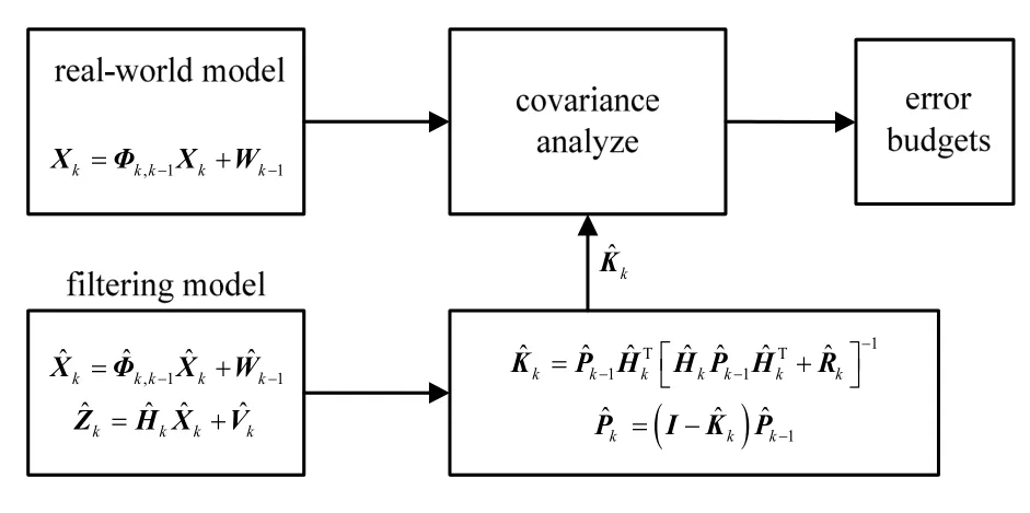
Fig.1 Calculation model of designed alignment covariance analyzing method
From fig.1 we can see that, two models are involved in covariance analyzing method, one is“real-world” model, which includes complete error sources in real, the description of this model always use a high dimension error vector and complicated random error equations. Whereas, in engineering, relatively low dimension error model and simpler random error equations considering computational efficiency and observability of states is used frequently. After filtering model and trajectory of aircraft alignment is obtained, filtering gain Kkcan be got at any measurement update moment theoretically. In fig1, the reason why notation of filtering gain represented with “^” is that the gain is calculated using designed error model rather than real-world model, which means it is not optimum. Substituting Kkinto real-world model, the real covariance matrix Pkcan be obtained using designed alignment covariance analyzing method. Eventually, error distributions of the desired state at any time point is available.
1 The designed covariance analyzing method
In fig1, “covariance analyze” part is the core of the whole method., considering the linearity of error propagation, any error states at any time point is composed of all error sources with different coefficients.

Obviously, what need to be done is to find a method to getat time point t. All the error propagation can be depicted using Kalman filtering covariance propagation equations
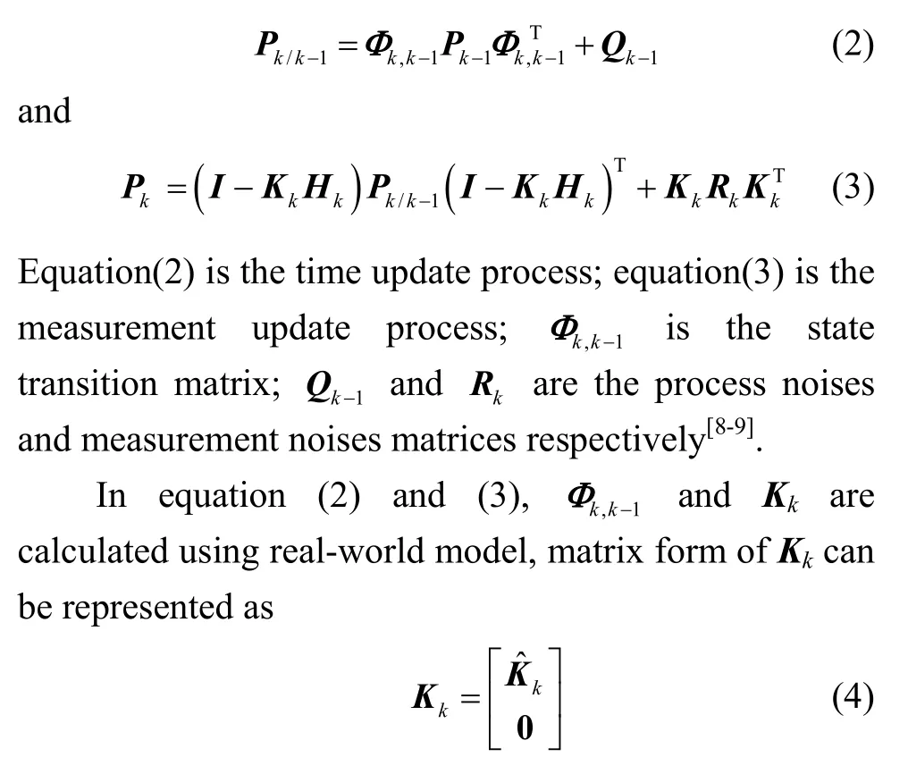
From equation (1), (2) and (3), it can be seen that“covariance analyze” part’s job is to separate propagation equations (3) and (4) into three distinguishing parts (initial errors, process noises and measurement noises). Obviously, when individual part of errors is analyzed, other two parts will not taken into consideration, and specific computational process of these three parts will be discussed next.
Considering that each part of errors can affect both time and measurement updates of filtering, both equation (3) and (4) will be included in all three error propagation equations.
1) Initial errors:
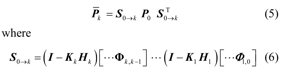
In equation(5), P0is the initial variance matrix of initial errors; S0→kis the transition matrix from timepoint 0 to k;Pkis the variance matrix at time point k caused by initial errors. It can be seen that both Qk-1and Rkare not showed in equation(6), P0is a strictly diagonal matrix, and φijis the ith row and jth column element of S0→k.
2) Process errors:
Taking account of gyros’ noise, the error propagation process is calculated using
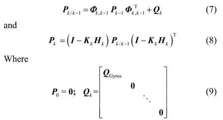
In equation(9), QGyrosis the variance matrix of gyros’noise, P0is set as zero matrix to make sure there’s no initial errors included. Unlike initial errors, process noises propagation processes will not be obtained by using equation(7) and (8) only once, which means the updating times of covariance matrices equal to the numbers of the process errors’ type.
3) Measurement errors:
Take GPS’s positioning noise for example, error propagation process is calculated using:
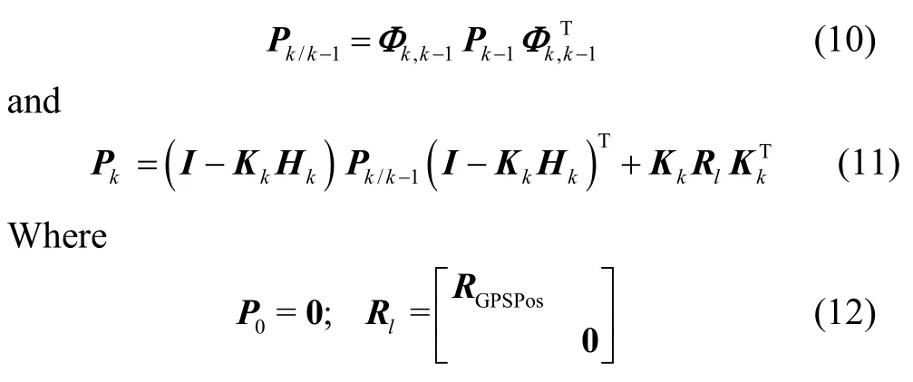
In equation(12), RGPSPosis the variance matrix of GPS’s positioning noise, measurement noises propagation processes will repeated as much as the numbers of the measurement errors’ type.
It can be seen that “covariance analyze” part essentially using variance propagation equations (equation (2) and (3)) to calculate different types of errors, whose calculation process can be obtained simultaneously.
2 Monte-Carlo simulation method
Error distributions can be easily and rapidly got using the designed covariance analyzing method, and next job should be adjusting mainly influenced errors to fulfill the precision requirement of in-flight alignment. Afterwards, it would be wise to testify the alignment result using Monte-Carlo simulation method. The reason why Monte-Carlo simulation should be applied is that error propagation process of strapdown inertial navigation is essentially non-linear, whereas, the covariance analyzing method can only evaluates the linear part. Monte-Carlo simulation method is an appropriate method to depict the characteristics of non-linearity, which means it can get a more correct analysis result of initial alignment process, and it can be used as a verification method for the designed covariance analysis method.
Monte-Carlo method also called statistics test method, not only can be used to solve some probability problem directly, but also some certainty problems[10]. The theoretical basis of this method is the law of large numbers: if the tests repeats N times under the same condition,the arithmetic mean value of observed random variable converges in probability at the value of expectation with N→∞.
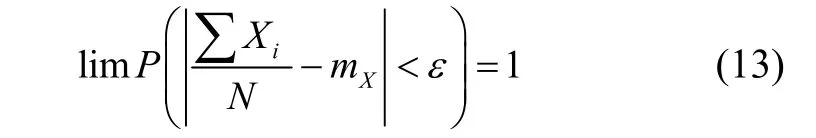
Where, Xiis the observed random variable; mXis the value of expectation; N is the numbers of tests. What Monte-Carlo method do is generating various samples, and each sample simulate one set of initial alignment test, the bigger the N is chosen, the higher the reliability of evaluation is.
One thing should bewared of is that Monte-Carlo method here is only treated as an evaluation tool of the designed covariance analyzing method, so it will only run once. Although Monte-Carlo method can be used to evaluate various error sources, it will take very long time to finish the task of error distributions.
3 In-flight alignment simulation and analysis
The rule of error propagation of inertial navigation system is not only related to IMU’s own error characteristics, but also related to aircraft’s maneuvering during alignment process. Different maneuvering may induce different impact on navigation precision. This section will study on error distributions of azimuth error angle ψ at the end of alignment process of three different flying maneuverings, and kinematic parameters of these trajectories are showed in fig.2.
In fig.2, total alignment time of trajectories is 10 min, and initial velocities is 150 m/s . Trajectory A keeps constant speed during alignment. Trajectory B and C accelerate during 20~30 s , and decelerating during 200 s~ 210 s , and acceleration modulus value of the trajec-tories are 1 m/s2and 3 g respectively. All trajectories’alignment time is 5 min. The purpose of introducing accelerating and decelerating move is to enhance the observability of azimuth error angle, thus the alignment precision is enhanced.
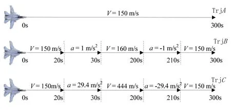
Fig.2 Trajectories of three different maneuverings
Refer to fig.1, in order to depict the system more accurately, a 45 dimension real-world model is built, the parameters are set in table.1.
In table.1, the word “accl” means accelerometer. The correlation time of gyros and accelerometers are set as 300 s and 7200 s, and gravity model error is depicted as 1-order Markov process with the correlation distance set as 20 nm. The integration mode of velocity and position is used in SINS/GPS in-flight alignment; filtering state has typical 15 dimension states with navigation errors and gyros’ and accelerometers’ constant biases, initial variance; process and measurement variances are appropriately magnified to guarantee the robustness. Initial azimuth angle is set as 45° with additive error of 35′ . Error distributions of azimuth error angle of the alignment processes at the end of these three trajectories is showed in table.2; comparison of designed covariance analyzing method and Monte-Carlo simulation method is showed in fig.3.

Fig.3 Azimuth error angle curves using the designed variance method and the MC method(200 times)
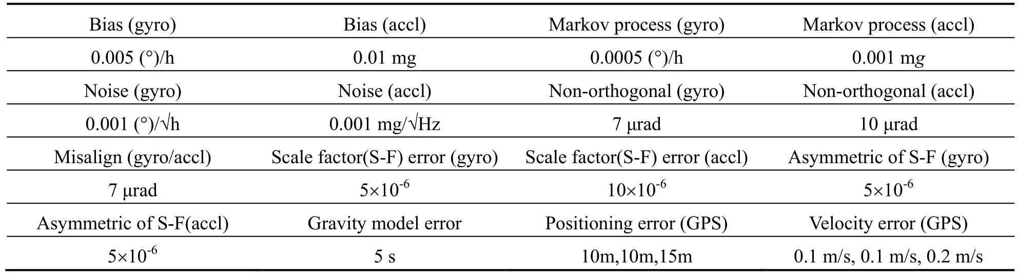
Tab.1 Parameter setting of the real-world IMU’s model

Tab.2 Error distributions of alignment processes at the end of the trajectories (unit: arcmin)
In table2, some error sources are merged for they may have similar characteristics. For instance, initial errors include initial attitude, velocity and position error. It can be seen that trajectory A , B, C have different error distributions because of the difference of the maneuverings. The gyro error’s effect under the condition of uniform motion is significantly higher than the trajectory with accelerated motion and decelerated motion, which can be seen from convergence curves in figure 3. It shows that acceleration maneuvering is indeed helpful to accelerate the convergence of azimuth error angle, and the azimuth angle’s estimated information is mainly from gyro under the condition of uniform motion. Therefore, in the relatively stable environment, gyro has much more effect to the result of azimuth alignment. Trajectory C and trajectory B accelerate and decelerate at the same period, but C with the acceleration module value reaching 3g, which improves the GPS’s velocity measurement signal-tonoise ratio further. At this time, the azimuth error introduced from GPS measurement noise is the smallest of the three trajectories. In addition, the effect of the azimuth error from gravity model error should be paid enough attention to. Obviously, to obtain the high precision initial attitude information from in-flight alignment, it is necessary to establish the accurate gravity model among the alignment period. Meanwhile, it can be seen from the table 2 and figure 3 that the results of variance analysis method correspond highly with the result of Monte-Carlo simulation, which show that the analyzing method is correct.
4 Conclusion
The designed covariance and the Monte-Carlo simulation method are used to solve the problem of error distributions of in-flight alignment. Three different trajectories are employed to testify the accuracy of the analysis method proposed in this paper, and result shows that the designed covariance and the Monte-Carlo simulation method are highly corresponded, which indicates that the method proposed here can be used for providing error distributions of in-flight alignment before real flight experiments.
[1] Acharya A, Sadhu S, Ghoshal T K. Improved self-alignment scheme for SINS using augmented measurement[J]. Aerospace Science and Technology, 2011, 15(2): 125-128.
[2] 林玉荣, 邓正隆. 基于矢量观测确定飞行器姿态的算法综述[J]. 哈尔滨工业大学学报, 2003, 35(1): 38-45. Lin Yu-rong, Deng Zheng-long. Summary of Algorithms for determination of spacecraft attitude from vector observations[J]. Journal of the Harbin Institute of Technology, 2003, 35(1): 38-45.
[3] 翁浚, 秦永元, 严恭敏, 等. 车载动基座FOAM对准算法[J]. 系统工程与电子技术, 2013, 35(7): 1498-1501. Weng Jun, Qin Yong-yuan, Yan Gong-min, et al. Vehicular moving-base FOAM alignment algorithm[J]. Systems Engineering and Electronics, 2013, 35(7): 1498-1501.
[4] Wu Feng, Qin Yong-yuan, Zhang Jin-liang. Interacting multiple model algorithm for SINS self-alignment on shipboard aircraft[C]//Proceedings of the 32nd Chinese Control Conference. Xi’an, China, 2013: 4937-4941.
[5] Adusumilli S, Bhatt D, Wang H, et al. A low-cost INS/GPS integration methodology based on random forest regression[J]. Expert Systems with Applications, 2013, 40(11): 4653-4659.
[6] 李增科, 高井祥, 姚一飞, 等. GPS/INS 紧耦合导航中多路径效应改正算法及应用[J]. 中国惯性技术学报, 2014, 22(6): 782-787. Li Zeng-ke, Gao Jing-xiang, Yao Yi-fei, et al. GPS/INS tightly-coupled navigation with multipath correction algorithm[J]. Journal of Chinese Inertial Technology, 2014, 22(6): 782-787.
[7] 胡高歌, 刘逸涵, 高社生, 等. 改进的强跟踪UKF算法及其在INS/GPS组合导航中的应用[J]. 中国惯性技术学报, 2014, 22(5): 634-639. Hu Gao-ge, Liu Yi-han, Gao She-sheng, et al. Improved strong tracking UKF and its application in INS/GPS integrated navigation[J]. Journal of Chinese Inertial Technology, 2014, 22(5): 634-639.
[8] Wu Mei-ping, Wu Yuan-xin, Hu Xiao-ping, et al. Optimization-based alignment for inertial navigation systems: Theory and algorithm[J]. Aerospace Science and Technology, 2011, 15(1): 1-17.
[9] Yan Gong-min, Zhou Qi, Weng Jun, et al. Inner Lever Arm Compensation and Its Test Verification for SINS[J]. Journal of Astronautics, 2012, 33(1): 62-67.
[10] Mei Chun-bo, Qiin Yong-yuan, You Jin-chuan. SINS in-flight alignment algorithm based on GPS for guided artillery shell[J]. Journal of Chinese Inertial Technology, 2014, 22(1): 51-57.
空中对准方案的误差分配分析方法
翁 浚,秦永元,严恭敏,梅春波
(西北工业大学 自动化学院,西安 710129)
舰载机进行紧急作战任务时,可能会先快速起飞,然后再进行空中对准。为了保证对准结束进入惯性导航模式后,惯导系统能够达到一定精度指标,对准结束时刻的姿态信息需要达到一定的精度要求。空中对准过程一般可分为粗对准和精对准两部分,对准结束时刻的姿态精度由粗对准结束时刻的导航误差、惯性器件误差、重力场模型误差和对准过程中的飞行机动等多个因素决定。首先利用设计的协方差分析方法,对两种不同空中对准方案进行误差分配,并通过 Monte-Carlo仿真技术对误差分配结果进行了验证。仿真结果说明了提出的误差分析方法是正确的,为空中对准方案的改进方向提供了借鉴作用。
空中对准;误差分配;协方差分析;蒙特卡洛仿真
V249.3
:A
2015-05-25;
:2015-09-15
国家自然科学基金资助(61273333)
翁浚(1988—),男,博士研究生,主要研究方向为惯性导航、组合导航。E-mail:npu_wengjun@sina.com
1005-6734(2015)05-0570-05
10.13695/j.cnki.12-1222/o3.2015.05.003
