Construction of crash prediction model of freeway basic segment based on interactive influence of explanatory variables

Wang Xiaofei Li Xinwei,2 Fu Xinsha Zhao Lixuan Liu Xiaofeng

(1School of Civil Engineering and Transportation, South China University of Technology, Guangzhou 510641, China)(2Guangzhou Expressway Co., Ltd, Guangzhou 510288, China)(3Guangdong Police College, Guangzhou 510230, China)(4Guangdong Traffic Group Co., Ltd, Guangzhou 510623, China)



Construction of crash prediction model of freeway basic segment based on interactive influence of explanatory variables

Wang Xiaofei1Li Xinwei1,2Fu Xinsha1Zhao Lixuan3Liu Xiaofeng4

(1School of Civil Engineering and Transportation, South China University of Technology, Guangzhou 510641, China)(2Guangzhou Expressway Co., Ltd, Guangzhou 510288, China)(3Guangdong Police College, Guangzhou 510230, China)(4Guangdong Traffic Group Co., Ltd, Guangzhou 510623, China)

In order to improve the prediction precision of the safety performance function (SPF) of freeway basic segments, design and crash data of 640 segments are collected from different institutions. Three negative binomial (NB) regression models and three generalized negative binomial (GNB) regression models are built to prove that the interactive influence of explanatory variables plays an important role in fitting goodness. The effective use of the GNB model in analyzing the interactive influence of explanatory variables and predicting freeway basic segments is demonstrated. Among six models, the two models (one is the NB model and the other is the GNB model.) which consider the interactive influence of the annual average daily traffic (AADT) and length are more reasonable for predicting results. Furthermore, a comprehensive study is carried out to prove that when considering the interactive influence, the NB and GNB models have almost the same fitting performance in estimating the crashes, among which the GNB model is slightly better for prediction performance.

crash; freeway; safety performance function (SPF); interactive influence of explanatory variables; generalized negative binomial (GNB)

Compared to other kinds of highways, the freeway is often designed with a relatively good driving environment, such as high alignment indices, a good pavement, being completely closed, no pedestrians, no interference from low speed, effective traffic safety devices, and so on. Thus, the accident rate and death toll on the freeway is within an average of 30% to 51% and 43% to 76% of ordinary highways in developed countries. However, the number of accidents, death tolls, injury tolls and the direct loss of property is 3.2, 8.4, 7.2 and 24.3 times the ordinary average for highways in China. Therefore, it is important to determine the actual circumstances of accidents occurring on freeways and how freeway environments influence the accident rates based on reliable databases.

Over the past several decades, historical surveys covering the characteristics and frequency of accidents involving freeways has been a very active research area[1-2]. However, in terms of freeway accidents in China, no specialized accident databases and highway design databases have yet been made available. Also, there is very little investigation clarifying China’s current situation. Zhong et al.[3-4]developed the crash prediction model with a relatively small number of samples. Therefore, this paper attempts to establish models with large samples.

Mathematical statistics and regression analysis have been common methods used in predicting highway crashes. Other methods, such as fuzzy mathematics, the grey theory, the nerve cell method and clustering analysis, have also been used to establish the prediction models. However, freeway accidents are the results of the combined influence of multiple factors, such as alignment, traffic volume, the presence of an interchange or other structures. The above-mentioned methods explain how a single factor influences the crashes but fail to explain the interactions between these factors and how these influence the crashes. For this reason, when studying the crash prediction models, the freeway is often divided into several segments (a basic segment, general segment and special segment). The prediction function of the basic segment is also called the safety performance function (SPF) and it is the basis of the others.

The parameters of the SPF are the length of the segment and the traffic volume. The prediction result is the number of crashes. As for general segments or special segments, the crash number can be modified by crash modification factors (CMFs). Thus, the SPF is the basis of the freeway crash prediction model and the precision of the final result will be directly determined by the SPF. In order to determine the combined influence of multifactors, flexibility is introduced here to explain the influence. Flexibility is used in the manufacturing industry to explain the variational environment or the probabilistic ability from the variation[5]. The Cobb-Douglas production function, the linear production function, the Leontief production function, the variable elasticity of substitution(VES)production function and the transcendental logarithmic (Trans-log) production function are often used to analyze flexibility[6-8]. Among these methods, the Trans-log production function is the most popular function used to analyze traffic problems. Thus, the Trans-log function is adopted in this paper to study the difference between the situations with and without considering the combined influence of multifactors. The model with the best fitting degree is chosen as the SPF. Then the SPF is checked by the real traffic accident data.

1 Model Format and Basic Segment Definition

In this paper, the model format is as[9]

Ne,x=NSPF,xCMFAADT,xCMFlane,x…CMFlight,x

(1)

whereNe,xis the predictive model estimate of the crash number for a specific year on site typex;NSPF,xis the predicted average crash number determined by the SPF on site typex; CMFAADT,x…CMFlight,xare the crash modification factors specific to site typex.

The basic segment for SPF is defined as follows.

Lane number: Two-way 4-lane;

Lane width: 3.75 m;

Hard shoulder: On both sides;

Median separator: Yes;

Crash barrier: On both sides;

Lighting: None;

AADT (two directions): No more than 5.76 (104pcu/d);

Open to traffic duration: No less than two years and no reconstruction in two years.

2 Data

In order to acquire sufficient samples for a meaningful statistical analysis, six major sources are used: the National Statistics Annual Report of Road Traffic Accidents (NSARRTA,2013)[10], the Statistical Bulletin of Transportation Industry Development (SBTID, 2013), accident data from the Traffic Management Committee of Guangdong Province (MCGP), accident data from different Traffic Police Detachments (TPD, 7 freeways, 593.099 km in total), accident data from different Freeway Administrations and Maintenance Centers accordingly(FAMC, 7 freeways, 593.099 km in total), and additional results provided by other scholars. As for the sample size, see Tab.1.

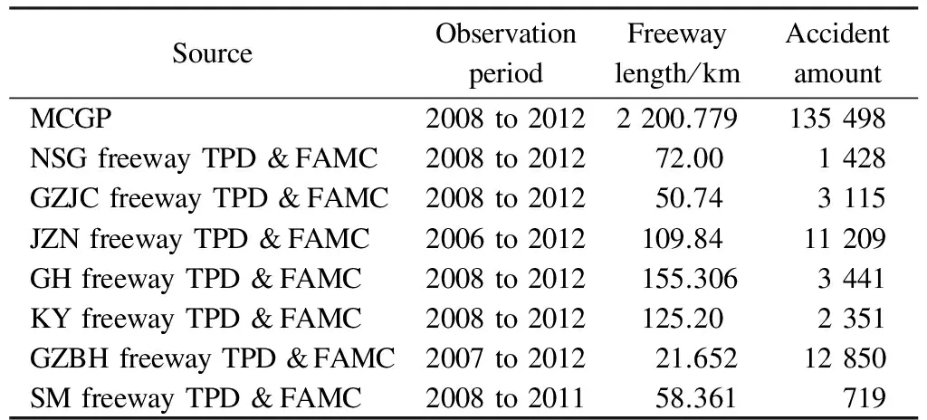
Tab.1 Sample source and size

3 Method

The basic function of the Trans-log NB production function is as follows[11-12]:

lnY=α0+αklnK+αLlnL+αkk(lnK)2+αll(lnL)2+αkllnKlnL

whereYis the dependent variable;K,Lare the explanatory variables; andα0,αk,αL,αkk,αll,αklare the estimated parameters.

In this paper, the annual average daily traffic (AADT)Qiand the segment lengthLiare chosen as explanatory variables. If not taking the influence between these two variables into consideration, the NB function is as follows:

lnμi+α0+α1ln(Qi)+α2ln(Li)

(2)

whereμiis the estimate of crash number for a specific year of segmenti;Qiis the AADT for a specific year of segmenti;αk(k=0,1,…,5) are the estimated parameters.

If taking the influence between these two variables into account, the trans-log NB function is as follows:

lnμi=α0+α1ln(Qi)+α2ln(L1)+α3[ln(Qi)]2+

α4[ln(Li)]2+α5ln(Qi)ln(Li)

(3)

Thus, six models are used as shown in Tab.2. Models 1 to 4 do not take the influence between two variables into account and Models 5 and 6 consider the influence. Models 1, 2 and 5 are NB regression models and others are GNB regression ones.

Tab.2 Models adopted and their estimated parameters

Note:βis the excessive dispersion coefficient of the NB or the GNB model.

Akaike information criterions (AIC)[13], Bayesian information criterions (BIC) and Pseudo R2 are adopted to test the accuracy of the prediction models. Cumulative residual and excessive dispersion coefficients are also used to evaluate the fit goodness of the models.

4 Analysis Process and Results

4.1 Models discussion

Estimated parameters which have been demarcated by survey data and parameters which reflect fit goodness have also been calculated. The results are listed in Tab.3.

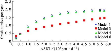
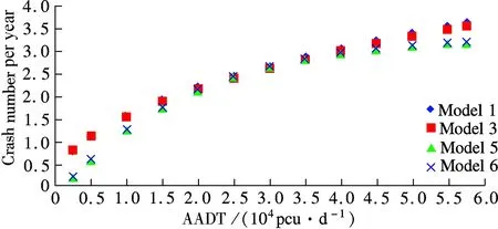
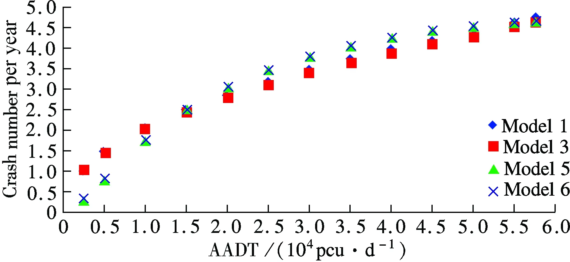
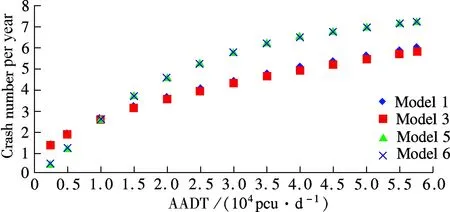
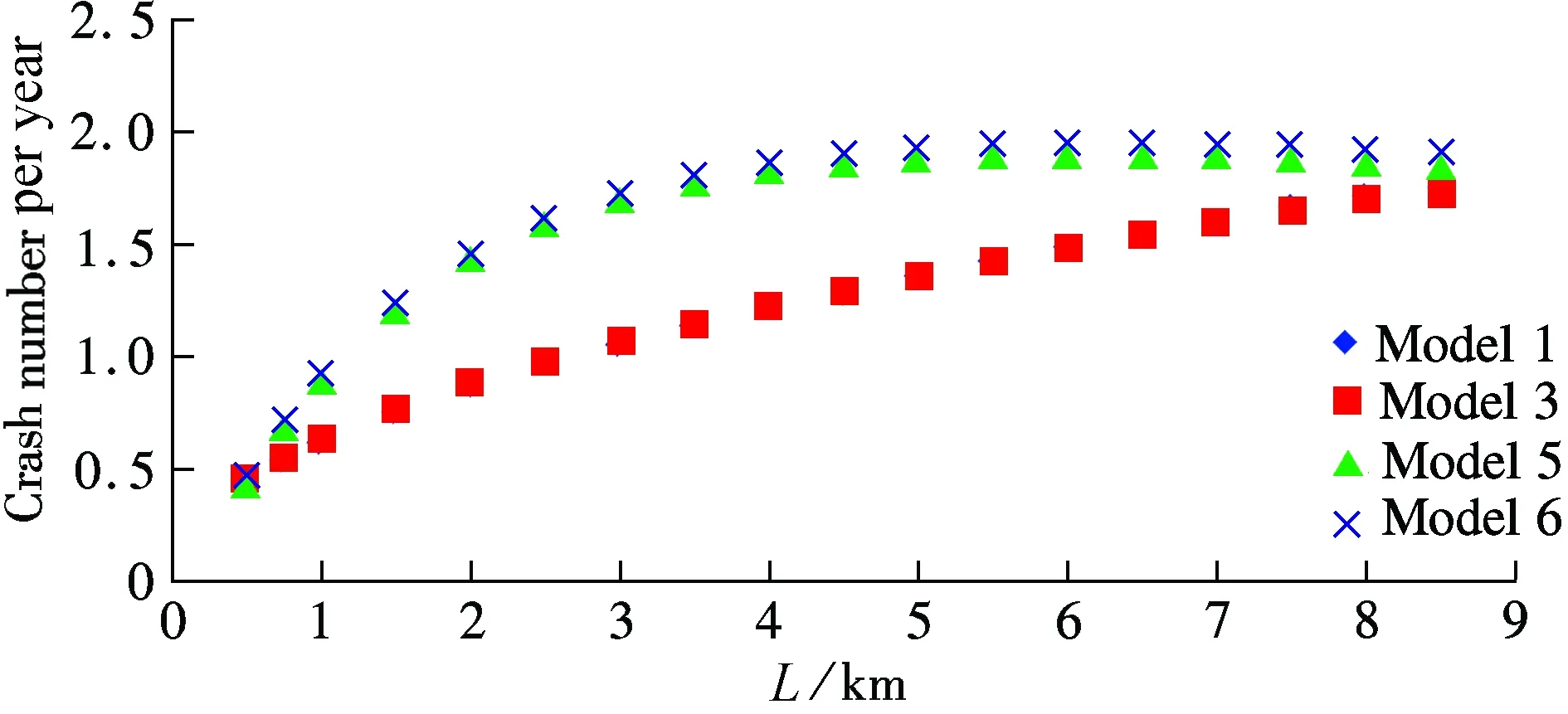
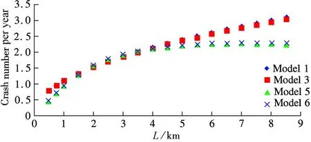
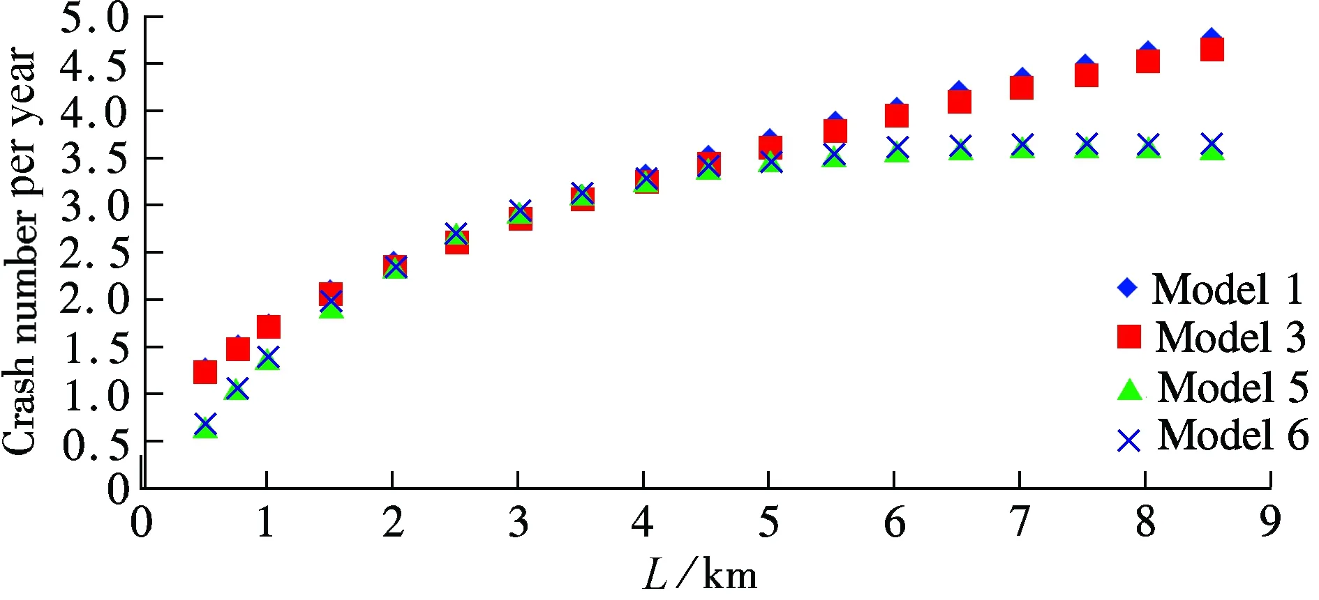
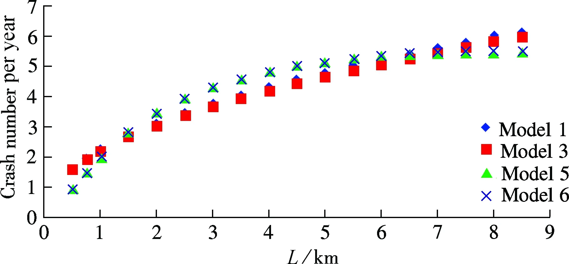
The results shown in Tab.3 indicate that the interactive influence between two variables is clear. Thus, Model 5 and Model 6, which take the interactive influence into consideration, have better fitting, particularly compared to Model 2 and Model 4. However, the fitting goodness difference among Models 1, 3, 5 and 6 is not very obvious, so further analysis is carried out to determine which one is more accurate. In the scope of the definition condition, the crash number can be predicted and the estimated results are shown in Fig.1 and Fig.2.

Tab.3 Estimated and statistical parameters

(a) (b)

(c) (d)

Fig.1 Variation tendency of estimated results with AADT under differentL. (a)L=0.5 km; (b)L=3.0 km; (c)L=5.0 km;(d)L=8.0 km

The results shown in Figs.1 and 2 show no difference between Models 1 and 3 or Models 5 and 6. As for Models 1&3 and Models 5&6, the results reveal a remarkable difference.

When the segment length is certain, crashes increase with AADT, as shown in Fig.1. The increase tendency shows that Models 5 and 6 have a clear increase with AADT when the AADT is less than 3.5×104pcu/d, however, the increase tendency is relatively gradual when AADT is more than 3.5×104pcu/d. In comparison with Models 5 and 6, the increase tendency of Models 1 and 3 appears to have uniform variations. The survey data shows that there is one point after which the tendency changes. This may be due to the fact that with the increase in the traffic volume, speed and driving space decrease, resulting in fewer crashes. Thus, Models 5 and 6 reveal a more accurate picture.

(a)

(b)

(c)

(d)

The results shown in Fig.2 with respect to segment length are not surprising. When AADT is certain, crashes increase with the segment length. The increase tendency also shows that Models 5 and 6 have a turning point at the length of 4.5 km. It reveals that the traffic flow tends to be steady in the same segment after several minutes’ driving. So, the crashes will not increase as much as before.

In conclusion, Models 5 and 6 show a good corroboration with actual reality. Thus, the prediction models, Model 5 based on NB regression and Model 6 based on GNB regression have taken the interactive influence into consideration much better than others.

4.2 Discussion of NB Model 5 and GNB Model 6

To examine these two models in more detail and test their accuracy, the cumulative residual and excessive dispersion coefficients are introduced to evaluate these two models.

1) Cumulative residual

Cumulative residual can be calculated by

(4)

Cumulative residuals will be centered at zero if the model fit is correct and the maximum threshold is the square root of the sample quantity, that is (-25.298, 25.298). Cumulative residuals can be used to test the above NB and GNB models. The results in Fig.3 show no difference between the two models. Most of the points are within the threshold scope and near thex-axis. Few residuals are less than the minimum threshold (-25.298). Thus, the two models are proved to be a good fit and show no difference between each other.

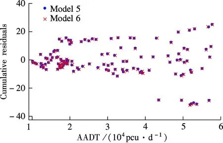
Fig.3 Cumulative residuals of Models 5 and 6

2) Excessive dispersion coefficientβ

The excessive dispersion coefficient of the NB model is constant and that of Model 5 is 0.337 3. As for the GNB, the excessive dispersion coefficient is the function of the explanatory variable lnL, which can be expressed as

β=e(λ0+λ1lnL)

(5)

whereλ0,λ1are the estimated parameters. In the example,λ0=-1.17,λ1=0.08. The regression results are shown in Tab.4 and Fig.4.

Further study discovers that the excessive dispersion coefficient of Models 5 and 6 are almost equal. It shows that the mean dispersion coefficient of Model 6 (0.332 0) is slightly better than that of Model 5 (0.337 3). In conclusion, testing by cumulative residual and excessive dispersion, the two models demonstrate a good fit and there is almost no difference. They can both be used as the SPF of basic segment. In this paper, Model 6 (GNB) is adopted as SPF for further study.

Tab.4 Statistical index of the excessive dispersion coefficient of Model 6

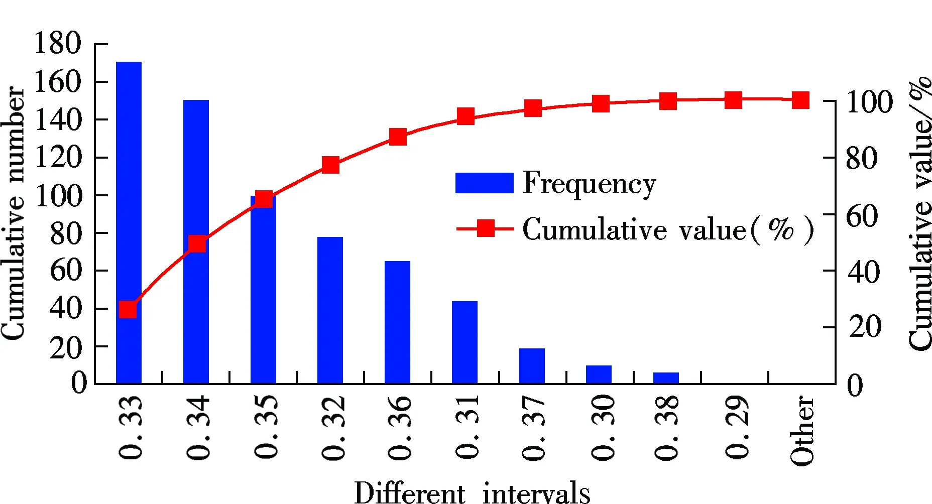
Fig.4 Excessive dispersion coefficients at different interval distributions of Model 6

4.3 Results

According to the above analysis, the following model is proposed as the freeway basic segment defined in Section 1:

NSPF,x=e[-0.11+0.85lnAADTx+0.09lnLx-0.22(lnAADTx)2+0.20(lnLx)2+0.06lnAADTxlnLx]

(6)

where AADTxis the AADT of basic segmentx, 104pcu/d;Lxis the length of basic segmentx, km.

In order to test the model, crashes estimated by Eq.(6) are compared with the actual data (see Tab.5). From Tab.5, it can be seen that the prediction crashes are very close to the actual values. It therefore proves that the SPF based on GNB can predict crashes correctly.

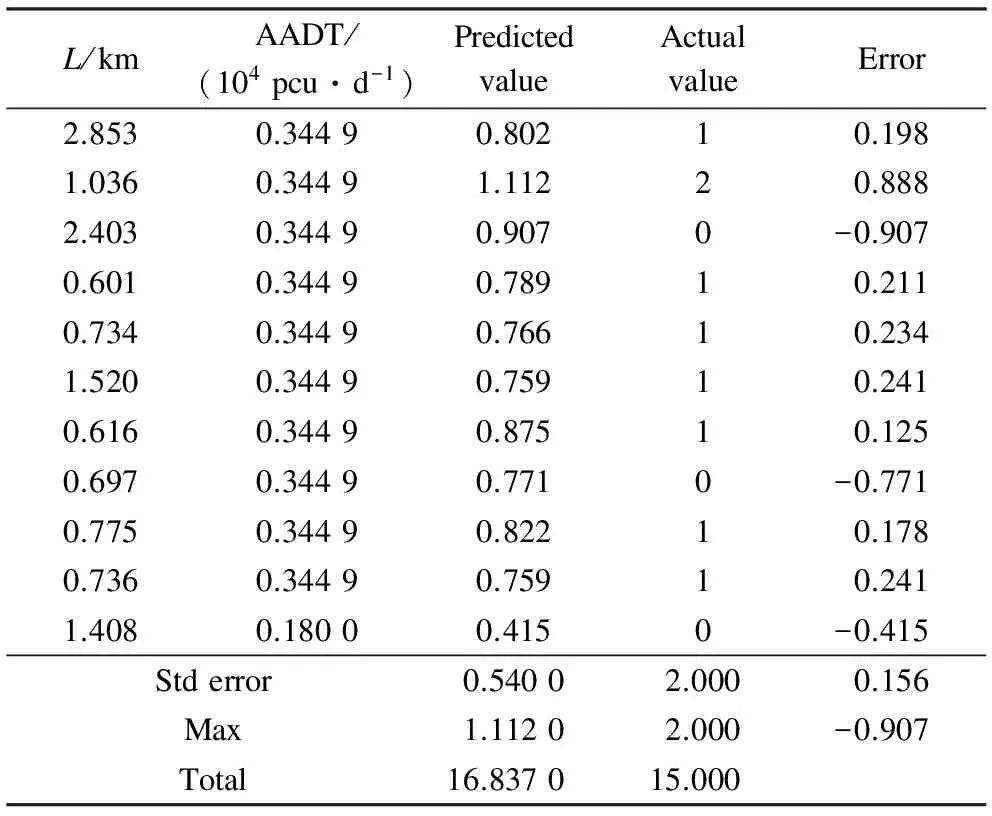
Tab.5 Comparison of the crashes estimated by Eq.(6) with the actual data

5 Conclusion

The analysis sheds light on the safety performance function (SPF) of the freeway basic segment. With detailed analysis and study, some conclusions are drawn as follows:

1) With enough samples and data, the effective use of the GNB model in analyzing the interactive influence of explanatory variables and predicting crashes on the freeway basic segment has been proved.

2) The contribution of interactive influence between the NB model and the GNB model is compared. The results show that when interactive influence is taken into consideration, the prediction results of the crash increase tendency becomes more accurate by using AADT or the length.

3) Furthermore, comprehensive study proves that when considering the interactive influence, the NB and GNB models have almost the same good fit when estimating the crashes, among which the GNB model is slightly better.

[1]Durduran S S. A decision making system to automatic recognize of traffic accidents on the basis of a GIS platform[J].ExpertSystemswithApplications, 2010, 37(12): 7729-7736.

[2]White J, Thompson C, Turner H. WreckWatch: automatic traffic accident and notification with smartphones[J].MobileNetworksandApplications, 2011, 16(3): 285-303.

[3]Zhong Liande. Research on accident prediction model of freeway [D]. Beijing, China: Key Laboratory of Traffic Engineering, Beijing University of Technology, 2008. (in Chinese)

[4]Ma Zhuanglin. Temporal-spatial analysis model of traffic accident and its prevention method on expressway [D]. Beijing, China: School of Traffic and Transportation, Beijing Jiaotong University, 2010. (in Chinese)

[5]Mandalbaum M. Flexibility in decision making:an exploration and unification [D]. Toronto, Canada:Department of Engineering, University of Toronto,1978.

[6]Wu Lurong, Liang Fangfang, Shi Zhikai. China’s trans-log production function model of losses of traffic accidents[J].MathematicsinPracticeandTheory, 2010, 40(22):56-61.

[7]Fridstrom L, Ifver J, Ingebrigtsen S, et al. Measuring the contribution of randomness, exposure, weather and daylight to the variation in road accident counts[J].AccidentAnalysisandPrevention, 1995, 27(1): 1-20.

[8]Zeng Juan. Research on influencing factors of socio-economic losses of road traffic accident based on generalized linear models[J].JournalofWuhanUniversityofTechnology, 2010, 32(6): 155-158.(in Chinese)

[10]Ministry of Transport of the People’s Republic of China. Statistical bulletin of communication and transportation industry development in 2013[EB/OL]. (2014-05-13)[2014-06-20]. http://www.moc.gov.cn/zfxxgk/bnssj/zhghs/201405/t20140513_1618277.html.(in Chinese)

[11]Christensen L R, Jorgenson D W, Lau L J. Transcendental logarithmic production frontiers[J].ReviewofEconomics&Statistics, 1973, 55(1):28-45.

[12]Li Rong, Liu Xiang, Liu Jian. Research on traffic accident frequency prediction based on translog production function[J].JournalofHunanUniversity:NaturalSciences, 2013,40(4):49-54.(in Chinese)

[13]Bozdogan H. Model selection and Akaike’s information criterion (AIC): the general theory and its analytical extensions[J].Psychometrika, 1987, 52(3):345-370.

基于变量相互影响的高速公路基本路段事故预测模型构建方法

王晓飞1李新伟1,2符锌砂1赵立萱3刘小峰4

(1华南理工大学土木与交通学院,广州 510641)

(2广州市高速公路有限公司,广州 510288)

(3广东省警官学院,广州 510230)

(4广东省交通集团有限公司,广州 510623)

为了提高基本路段事故预测模型(SPF)的预测精度,收集了640个基本路段设计资料及事故资料,应用3个负二项回归模型(NB)和3个广义负二项(GNB)回归模型对收集的数据进行拟合,并分析了解释变量的交互影响.研究表明在上述6个模型中,其中考虑了年平均日交通量和路段长度交互影响的2个模型(一个为NB，另一个为GNB),其预测结果更为合理.进一步综合对比表明考虑交互影响时,NB模型和GNB模型的适用性几乎相同,而GNB略佳.

事故;高速公路;事故预测模型;解释变量交互影响;广义负二项模型

U412.3

Foundation items：The National Natural Science Foundation of China (No.51408229,51278202), the Program of the Key Laboratory of Road and Traffic Engineering of the Ministry of Education, Tongji University (No.K201204), the Science and Technology Program of Guangdong Communication Department (No.2013-02-068).

：Wang Xiaofei, Li Xinwei, Fu Xinsha, et al. Construction of crash prediction model of freeway basic segment based on interactive influence of explanatory variables[J]．Journal of Southeast University (English Edition),2015,31(2):276-281．

10.3969/j.issn.1003-7985.2015.02.021

10.3969/j.issn.1003-7985.2015.02.021

Received 2014-11-21．

Biography：Wang Xiaofei(1980—),female,doctor, lecturer, xiaofeiw@scut.edu.cn.