Retrieval and analysis of sea surface air temperature and relative humidity*
2015-02-15WuYumei伍玉梅HeYijunShenHui
Wu Yumei (伍玉梅), He Yijun, Shen Hui
(*Key Laboratory of East China Sea & Oceanic Fishery Resources Exploitation and Utilization, Ministry of Agriculture,East China Sea Fisheries Research Institute, Chinese Academy of Fishery Sciences, Shanghai 200090, P.R.China)(**Nanjing University of Information Science & Technology, Nanjing 210044, P.R.China)(***Institute of Oceanology, Chinese Academy of Sciences, Qingdao 266071, P.R.China)
Retrieval and analysis of sea surface air temperature and relative humidity*
Wu Yumei (伍玉梅)*, He Yijun***, Shen Hui***
(*Key Laboratory of East China Sea & Oceanic Fishery Resources Exploitation and Utilization, Ministry of Agriculture,East China Sea Fisheries Research Institute, Chinese Academy of Fishery Sciences, Shanghai 200090, P.R.China)(**Nanjing University of Information Science & Technology, Nanjing 210044, P.R.China)(***Institute of Oceanology, Chinese Academy of Sciences, Qingdao 266071, P.R.China)
Air temperature and relative humidity have been the main parameters of meteorology study. In the past data could be obtained from in-situ observations, but the observations are local and sparse, especially over ocean. Now we can get them from satellites, yet it is hard to estimate them from satellites directly so far. This paper presents a new method to retrieve monthly averaged sea air temperature (SAT) and relative humidity (RH) near sea surface from satellite data with artificial neural networks (ANN). Compared with the observations in Pacific and Atlantic, the root mean square (RMS) and the correlation between the estimated SAT and the observations are about 0.91℃ and 0.99, respectively. The RMS and the correlation of RH are about 3.73% and 0.65, respectively. Compared with the multiple regression method, the ANN methodology is more powerful in building nonlinear relations in this research. Thus the global monthly average SAT and RH are retrieved from the fixed ANN network from July 1987 to May 2004. In general the annual average SAT shows the increasing trend in recent 18 years. The abnormality of SAT is decomposed with the empirical orthogonal function (EOF). The leading three EOFs could explain 84% of the total variation. EOF1 (76.1%) presents the seasonal change of the SAT abnormality. EOF2 (4.6%) is mainly related with ENSO. EOF3 (3.3%) shows some new interesting phenomena appearing in the three main currents in Pacific, Atlantic and Indian Ocean.
sea surface air temperature, relative humidity(RH), artificial neural network(ANN), empirical orthogonal function(EOF)
0 Introduction
Air temperature (SAT) and humidity (RH) near sea surface have been the main parameters in the climate study and the important indices of interaction between ocean and atmosphere. It is helpful to study and protect our environment. But we know little about it yet, for data are sparse over ocean. Now it is considered to be a good alternative to obtain knowledge over ocean via satellites. Air temperature and humidity are difficult to be estimated from satellite data directly so far, for the physical principles among them are not known clearly. Ref.[1] presented a multivariable linear regression equation of SAT with AMSU-A brightness temperatures from the 52.8GHz and 53.6GHz channels and satellite-derived sea surface temperatures. In Ref.[2] the relationship between the Bowen ratio and sea-air temperature difference under unstable conditions over sea was obtained. Ref.[3] presented an exponential pattern to derive real-time SAT and RH from NOAA TOVS data. Other statistical methods were also developed[4-6]. These years artificial neural networks (ANN) methods were applied more and more in this field[7-10].
The empirical orthogonal function (EOF) is one of the effective methods in meteorology and oceanography, which could help to decompose some complicated oceanographic and meteorological phenomena into independent temporal and spatial modes. EOF was applied to analyze the variations of SST in Delaware bay[11]. In Ref.[12] EOF was applied to analyze global patterns of monthly mean anomalies of atmospheric mass with medium-range weather forecasts re-analysis. In this research, EOF is applied to analyze the main changes of the long-term retrieved SAT.
Although methods in the derivation of SAT and other parameters have been developed for many years, their accuracies still need to be improved. Meanwhile most researches were focused on the tropical zone or a small local area before. This research means to extend the scope of research to the global and only satellite data are used here. Data with higher spatial resolution and longer time-series are applied to this approach, which is developed based on Ref.[8]. The Long-term and large-scale satellite data are collected to retrieve the monthly average SAT and RH from satellite data by ANN method. The advantages of ANN are shown by the comparison with a nonlinear regression function. Furthermore the fixed ANN network is used to estimate the SATs during 1987-2004. Then the surface air temperature anomaly data (SATA) are calculated and EOF is adopted to analyze the main variation of the SATA.
1 Data
There involve two main kinds of data: the satellite data and the in-situ observations, which are processed to build and evaluate retrieval models. The satellite data are the inputs for retrieval models, which include monthly averages of wind speed (WS), atmospheric water vapor (AWV), liquid cloud water (LCW), rain rate (RR) and sea surface temperature (SST). The preceding four inputs are obtained by the special sensor microwave imager (SSM/I). The spatial resolution of grid is 0.25° latitude ×0.25° longitude. The fifth input is derived from advanced very high resolution radiometer (AVHRR) (4km×4km resolution). The record of data spans from July 1987 to May 2004. The in-situ observations, provided by tropical atmosphere ocean project (TOGA-TAO) and national data buoy center (NDBC), are used to develop and test the approach. TOGA-TAO is combined with TAO and PIRATA moored buoys, almost 80 buoys positioned along the equator between 10° S and 10° N. The period of TOGA-TAO data is from July 1987 to May 2004, so there are 203-months observation data for research. The data from NDBC are provided by 240 buoys/stations from July 1987 to December 2003. Their positions are mostly distributed from middle latitude to high latitude (Fig.1). The real-time measurement arrays of air temperature over ocean are used to compute the monthly averages. Because the numbers of available observations vary widely, the data are averaged according to the cutoff criterion of at least 20 observations to compute the monthly average[7]. The nearest satellite data are chosen to match with the in-situ data in the range of 0.3° centered on the observation positions. The dew temperatures observed by NDBC have to be transformed into relative humidity in order to consist with TOGA-TAO data. The statistical function is adopted as
RH=100×exp[(td-ta)×0.0623832]
(1)
wheretdandtaarethedewpointtemperatureandtheairtemperature,respectively,RHisthecorrespondingrelativehumidity.
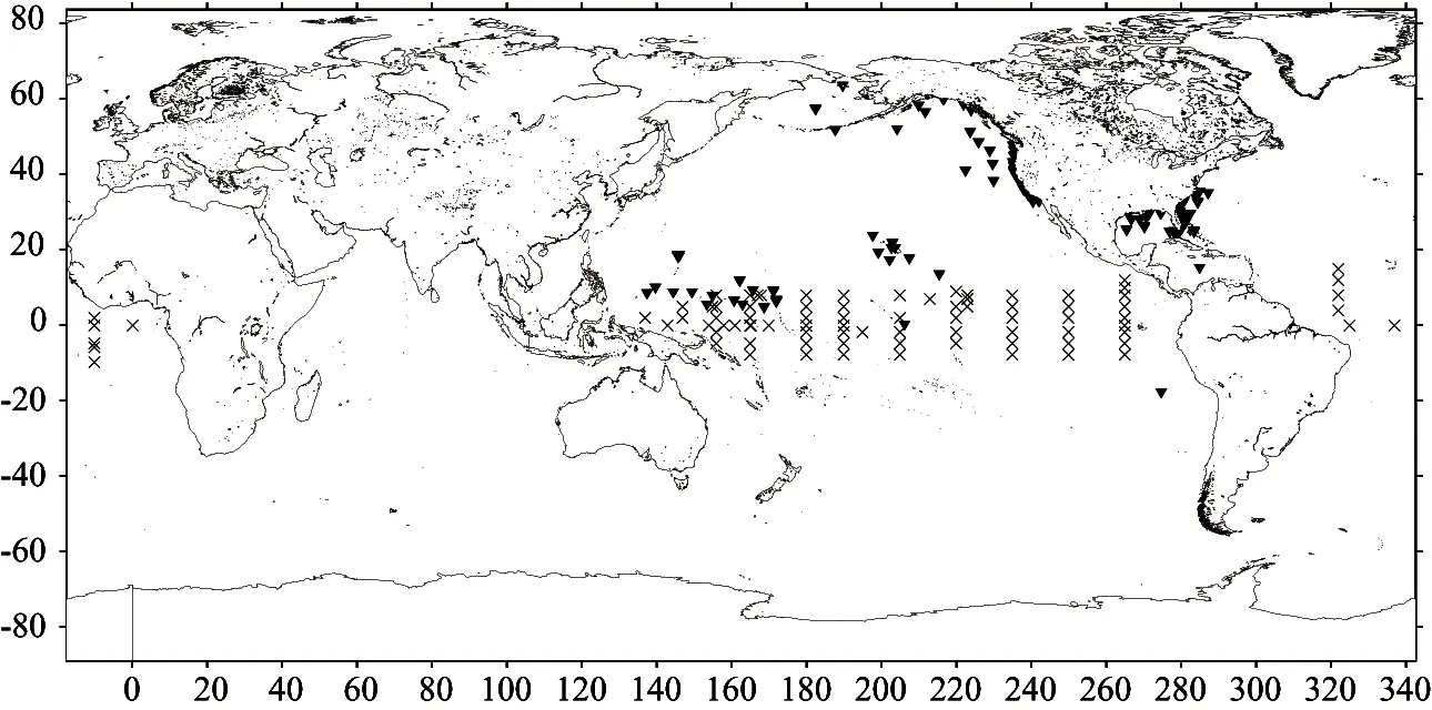
Fig.1 Spatial distributed plot of the observations. The crosses denote the locations of the moored buoys/stations in the NDBC domain. The triangles represent the locations of the moored buoys from TOGA-TAO. The website is http://www.ndbc.noaa.gov/.
After the process, there get 16,655 items meeting the cutoff criterion for SAT retrieval from July 1987 to May 2004. For there are few buoy/station observations with RH observation in 1980s, there are only 7,980 items for RH retrieval from February 1989 to May 2004. To build the ANN retrieval network, the SAT and RH data are divided into two parts according time, sample-Ⅰfor developing and training and sample-Ⅱfor simulating and validating. For SAT, sample-Ⅰincludes 8,482 items from July 1987 to May 1997 and sample-Ⅱ includes 8,173 items during June 1997 - May 2004. For RH, sample-Ⅰincludes 4,224 items from February 1989 to March 1999 and sample-Ⅱincludes 3,756 during April 1999 - May 2004.
2 Methodology
2.1 ANN method
The back-propagation neural network (BP NN) is adopted in this research. The ANN architectures for SAT and RH retrieval are designed as 4-10-4-1x and 5-13-4-1x, respectively. In the architecture of SAT retrieval, there includes four input parameters (AWV, LCW, WS and SST), 10 nodes in the first hidden layer and 4 nodes in the second hidden layer and one output (SAT). For RH network, there are five inputs (AWV, LCW, WS, RR and SST), two hidden layers (13 nodes in the first layer and 4 nodes in the second layer) and one output (RH). ‘x’ indicates the biases nodes associated with each hidden layer and the output. Sample-Ⅰ subset is input to the corresponding architecture to train the network. The back-propagation algorithm of Levenberg-Marquardt is chosen to adjust the weights of the network[12]. Once the BP NN fulfills the training targets, the network is fixed and sample-Ⅱ subset is used to test it. Several trainings are done and the network with the best accuracy is chosen for retrieve the global monthly mean SAT in the further.
2.2 Multiple regression method
ANN algorithms are powerful mathematical techniques in representing nonlinear relationships among a set of parameters. To validate it, a nonlinear regression function is built to compare with the ANN method. The estimation of SAT is taken as an example. The same data set as used in the ANN training (sample-Ⅰ8,482 data sets) is applied to fit a multiple nonlinear regression function (MNR) as
SAT=a0+a1W+a2V+a3C+a4SST+b1W2+b2V2+b3C2+b4SST2
(2)
whereparametersofW,V,CandSSTrepresentWS,AWV,LCW,andSST,respectively.ThecoefficientsinthefunctionareshownasTable1.

Table 1 Values of coefficients
2.3 Empirical orthogonal function method
Empirical orthogonal function (EOF) is one of the important statistical methods, which is widely used in meteorology. The matrix could be decomposed into a series of ranked eigenvectors with EOF, each of which could explain the total variation percentage[13,14]. In this research, EOF is applied to decompose SATA from 1987 to 2004 in order to find their main variations and causes. The leading eigenvectors are the emphases, which imply most of the total variation. The corresponding spatial modes and temporal series could be recognized to be related with some physical phenomena.
3 Result and analysis
3.1 Accuracy and comparison
Here the sample-Ⅱ dataset observed from TAO and NDBC are taken as the standard. The results of SAT and RH from ANN are compared with them. Fig.2 shows the scattered plot of SAT and RH from ANN with the independent testing items. In Fig.2(a), the RMS and the correlation of SAT are 0.91℃ and 0.99, respectively. Small bias is obtained. The estimations are equal or nearly equal to the observations. In Fig.2(b), the RMS and the correlation of RH are 3.73% and 0.65, respectively. There is a relatively large difference between the ranges of them. The scope of observations is [60%, 100%], but the retrieval result centralizes in the range of [68%, 93%]. The accuracies differ greatly in different areas. The better results observed in the low latitude [25°S, 25°N], the RMS of SAT and RH are 0.53℃ and 2.03%, respectively. The bigger error at the high latitude domain, the RMS for SAT is 1.06℃ and for RH 3.85%. There are two main reasons for the big bias in high latitude: (1) sparse in-situ data, (2) affection by the climate and the terrain. Only 5,154 SAT and 1,025 RH in-situ data are distributed at the high latitude domain. It is difficult for us to find exact estimations with sparse observations. Most of in-situ data distribute in the gulf or near the coast. Parameters around nearshore derived from satellite, especial SST and wind, are bigger errors than those over open oceans so errors of inputs may be passed to the estimations. Meanwhile the complicated weather in high latitude makes it difficult to obtain the accuracy as high as in low latitude. The accuracy of estimations is different in different seasons. The big errors mainly happen in the period from October to January, especially in January (not shown). In winter cold snaps happen frequently and the weather is unstable. Thus it brings bigger errors in unstable condition.

Fig.2 (a) Scattered plot of the monthly average SAT from ANN methodology and the observations. (June 1997~May 2004, n=8173 observations). (b) Scattered plot of the monthly mean RH from ANN and the observations. (April 1999~May 2004, n=3756 observations)
In order to illuminate the advantage of ANN, the results from ANN are compared with those of the MNR method. Fig.2 and Fig.3 show the results from ANN and MNR, respectively. The root mean square (RMS) of SAT between MNR and observations is 1.0℃ and the correlation is 0.99 (Fig.3). The RMS and the correlation between the ANN and the observations are 0.91℃ and 0.99, respectively (Fig.2(a)). Most of the results from these two methods agree well with in-situ data, except the cases of low temperatures. There appear larger errors in MNR than that in ANN in the cases below 3℃. The bias of ANN method is less than that of MNR and the correlation of ANN is a little higher. It is evident that the ANN methodology is more powerful in nonlinear simulations than the MNR method. Thus ANN methodology is chosen to retrieve global SAT and RH parameters. In the following parts, the results from ANN would be presented in detail.
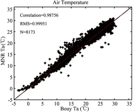
Fig.3 Scatter plot of the monthly average SAT from multiple nonlinear regression method and the observations from June 1997 to May 2004 (n=8173 observations)
3.2 SAT and RH retrieved from ANN
The above comparisons in the TAO and NDBC domains indicate that satellite data could act as an efficient alternative to estimate SAT and RH over open oceans by ANN. The global monthly mean SAT and RH from July 1987 to May 2004 are derived from the fixed ANN networks. Fig.4 presents two cases of global SATs retrieved from ANN, one is for the normal and the other is the warm case. Fig.4(a) is the estimation in January 2003. The SATs distribute regularly from north to south. The values of SAT in the south hemisphere are higher than that in the north on the same latitude, which is consistent with the seasonal feature. The cold tongue along the western coast of South America, the warm pool in the Indian Ocean and western Pacific Ocean are well presented in the SAT figures, for there is high relativity between SAT and SST. This conclusion agrees with that of Jones et al. (2003). Fig.4(b) shows the results derived in January 1998, when strong El Nio happened. We could see the SATs are higher in this warm case than that in the normal, especially that at low latitudes. The cool tongue along the western coast of South America almost disappears and there the cool tongue is replaced by warm water. It means some information of ENSO could be detected by observing air temperature like that from sea surface temperature.
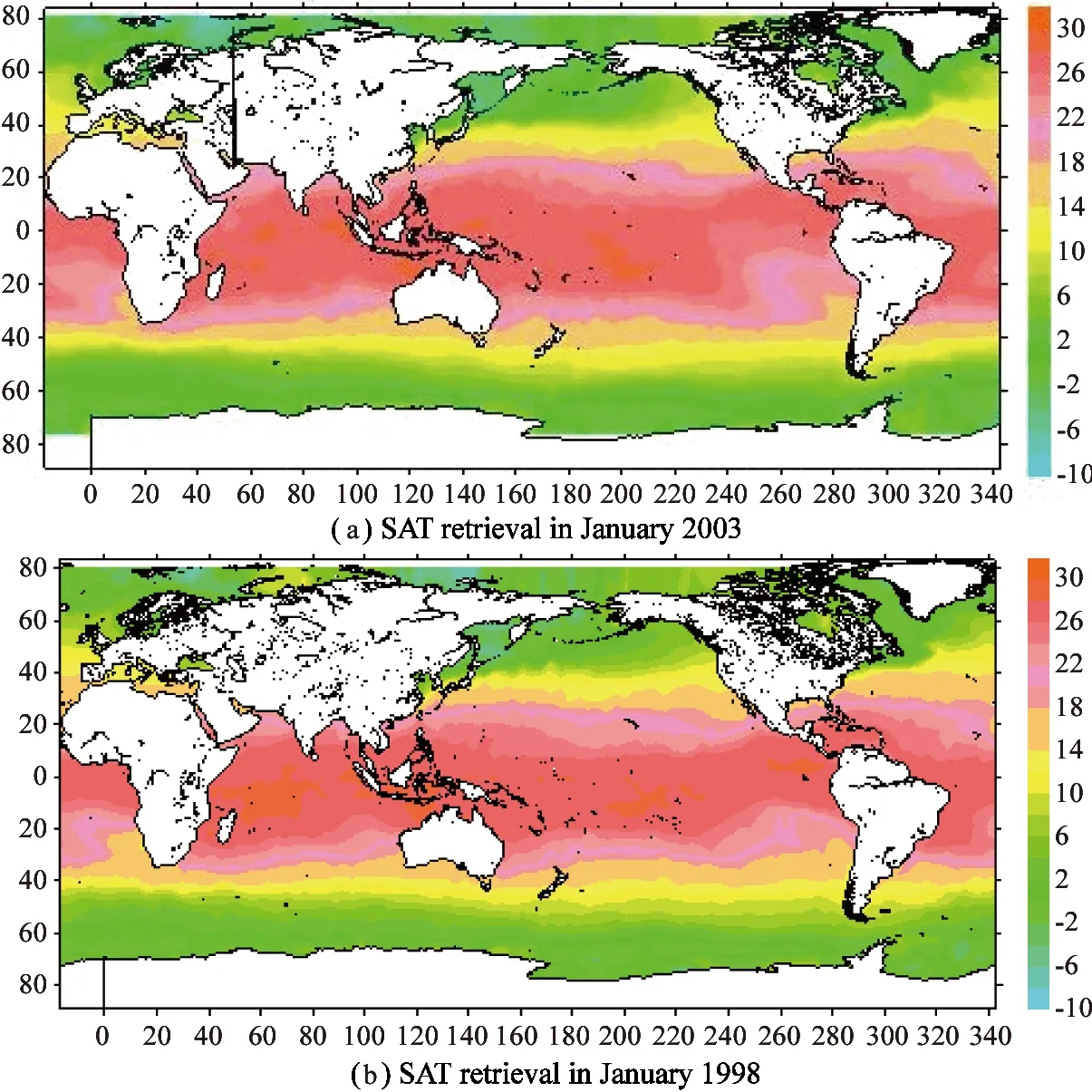
Fig.4 Monthly mean air temperature near sea surface derived from ANN method.The magnitude is shown by the greyscale bar of the image.
3.3 Analysis of SAT with EOF
The annual average SAT is undulate during the period of 1988~2003 (Fig.5). The highest value of annual average SAT (14.57℃) appears in 1998, when the strong El Nio happened. The lowest (14.25℃) appears in 1989 when the La Nia happened. When the values of SAT are averaged per five years, the increasing trend appears obviously with the ratio of 0.166℃/decade. The result is consistent with the global warming. However, we could not confirm the final trend for there are no enough data.
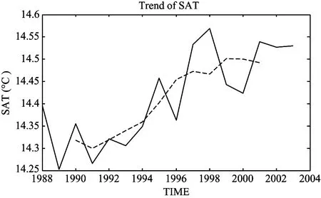
Fig.5 Trend of the annual averaged SAT from 1988 to 2003. The line denotes the annual average SAT. The dashed line represents the SAT after averaged per five years.
In order to find the main variation of SAT these years, EOF is applied to decompose the SAT anomaly matrix. As stated above, the monthly averages SAT from July 1987 to May 2004 have be retrieved from ANN. Then they are arranged into a two dimensional data matrix according to the time. Some location will be eliminated once its SAT value is absent in some month. After processed, the matrix of 43073×203 is got, where 43073 is the number of spatially distributed locations and 203 is the length of samples. In order to analyze the abnormal variability of SAT, the long-term average SAT is subtracted from the SAT to get surface air temperature anomaly (SATA). Thus EOF is applied to decompose the SATA matrix. The leading three eigenvectors and their EOFs are obtained. The results are presented in Table 2. The leading three EOFs could explain 84% of the total variance (figure not shown). The first EOF (EOF1), which accounts for 76.1%, mainly represents the seasonal variation of SAT. The shape of temporal series is similar to the curve of sine function and the period is almost one year. The opposite seasonal signs with out of phase over the two hemispheres are well shown. The corresponding time series show negative anomalies occur in boreal winter while positive in austral summer. It could be considered that EOF1 mainly accounts for the SAT variation affected by the seasonal change.
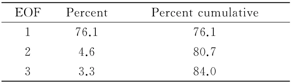
Table 2 Variances explained by EOFs
The second EOF (EOF2) explains 4.6% of the variances. It is found that in the temporal series of EOF2 a high peak appears during the El Nio period of 1997/1998. Combined with the corresponding spatial mode, large-scale high positive anomalies appear along the equator in eastern Pacific, where it should be cool in normal state. The maximum value of positive anomaly is up to 0.026℃. Meantime in western Pacific the SATAs are negative. They are out of phase between the eastern and western in Pacific from 0°S to 22°S. Perhaps EOF2 explains the contribution of ENSO to the anomaly of SAT over oceans.
In the spatial pattern of EOF3, we find that there are some similar phenomena of SATA over three oceanic currents: Kuroshio in Pacific, Gulf Stream in the west of Atlantic and Mozambique current in the west of Indian Ocean. The SATAs are opposite on the two sides of these currents. Negative anomalies appear to the south of these currents while positive anomalies emerge to the north. The area of anomaly affected by Gulf Stream is larger than that of Kuroshio, for the volume of the former is larger than that of the latter. These phenomena are worthy to be further studied. Over the waters of 30°S~51°S, the positive and negative SATAs appear by turns. This phenomenon is very like the spatial distribution of the Antarctic Circumpolar Current, which was described in Ref.[15]. In the area from 38°N to 58°N, there are large-scale positive anomalies. It can be thought that maybe the global warming phenomenon is more obvious in high latitude of the northern hemisphere these years.
4 Conclusions
A method of ANN is developed to retrieve monthly average SAT and RH from satellite data. It is managed to deal with the problems of sparse observations over ocean. Compared with the MNR method, ANN methodology is more powerful in establishing nonlinear relations in this field, especially in the case of low SAT. Compared with the in-situ data from TAO and NDBC, the RMS of SAT and RH from ANN are 0.91℃ and 3.73%, respectively. In the lower latitude, the accuracies are better and the RMSs are improved to 0.53℃ (SAT) and 2.03% (RH). The accuracy of SAT in low latitude is equal to that obtained by Jones et al.[8], which is known as the best accuracy so far. Although the accuracy of RH is not as good as that of SAT, a new experiment is shown here for further research. The main obstacle is the lack of observations, especially in the high latitude. More in-situ data are needed in the further research to find the relation and improve the accuracy.
The above analysis shows the ability of ANN to extract the accurate results of SAT and then the SATs retrieved from 1987 to 2004 are analyzed. The annual average of SAT shows an increasing trend in the recent 18 years. The SATAs are decomposed by EOF. The leading three eigenvectors could explain 84% of the total variances. The annual variability is the dominant, which is showed by EOF1 (76.1% of variance). It means that SATAs are mostly affected by the solar irradiation. ENSO phenomena could be found from EOF2. The biggest positive anomaly happens in the eastern Pacific during the strong El Nio of 1997/98. The least appears in the La Nia of 1989. In EOF3 spatial pattern, there is a large scale positive SATA in the high latitude area. It could be accounted for that the warming phenomena mainly appear in the high latitude. This result is close to the conclusion in Ref.[16], which indicates that the global air temperatures are warming in the recent decades and positive anomalies mostly happen in the high latitudes on the northern hemisphere. It is surprising that the SATAs are out of phase on the two sides of the three currents of Kuroshio, Gulf Stream and Mozambique current. The positive anomalies happen to the north of these currents and negative to the south. It may be the currents’ responses to the global warming. It is encouraged that the signal of SATA could imply the information of the Antarctic Circumpolar Current. It may be taken as a favorable evidence as the Antarctic Circumpolar Current. Here we only tell the phenomena resulted from EOF, while its causes and validations are not included.
[1] Jackson D L, Wick G A. Near-surface air temperature retrieval derived from AMSU-A and sea surface temperature observations.JournalofAtmosphericandOceanicTechnology, 2010, 27: 1769-1776
[2] Hsu S A. A relationship between the Bowen ratio and sea-air temperature difference under unstable conditions at sea.JournalofPhysicalOceanography, 1998, 28: 2222-2226
[3] He Y J, Wu Y M, Zhang B, et al. Near sea surface air temperature estimated from NOAA data. In: International Geoscience and Remote Sensing Symposium, Seoul, Korea, 2005. 3: 1485-1488
[4] Thadathil A, P, Shikauchi A, Sugimori Y, et al. A statistical method to get surface level air-temperature from satellite observations of precipitable water.JournalofOceanography, 1993, 49: 551-558
[5] Kubota M, Shikauchi A. Air temperature at ocean surface derived from surface-level humidity.JournalofOceanography, 1995, 51: 619-634
[6] Liu C C, Liu G R, Chen W J, et al. Modified Bowen ratio method in near-sea-surface air temperature estimation by using satellite data.IEEETransactionsonGeoscienceandRemoteSensing, 2003, 41(5): 1025-1033
[7] Gautier C, Peterson P, Jones C. Ocean surface air temperature derived from multiple data sets and artificial neural networks.GeophysicalResearchLetter, 1998, 25(22): 4217-4220
[8] Jones C, Peterson P, Gautier C. A new method for deriving ocean surface specific humidity and air temperature: an artificial neural network approach.JournalofAppliedMeterology, 1999, 38: 1229-1245
[9] Wu Y M, He Y J, Meng L. Monthly mean near sea surface air temperature and humidity retrieved from satellite data.OceanologiaEtLimnologiaSinica, 2008, 39(6): 547-551
[10] WU X R, Han G J, Zhang X F, et al. Retrieving near-surface air temperature in the South China Sea using artificial neural network.JournalofTropicalOceanography, 2012, 31(2): 7-14
[11] Keiner L E, Yan X H. Empirical orthogonal function analysis of sea surface temperature patterns in Delaware bay.IEEETransactionsonGeoscienceandRemoteSensing, 1997, 35:1299-1306
[12] Wen X, Zhou L, Wang D L, et al. Application and Design of Artificial Neural Networks in MATLAB. Beijing: Science Press, 2002. 207-232
[13] Zhao J P. Improvement of the mirror extending in empirical mode decomposition method and the technology in eliminating frequent mixing.HighTechnologyLetters, 2002, 8: 40-47
[14] Trenberth K E, Stepaniak D P, Smith L. Interannual variability of patterns of atmospheric mass distribution.JournalofClimate, 2005, 18 (15): 2812-2825
[15] Zhou Q, Zhao J P, He Y J. Low-frequency variability of the Antarctic Circumpolar Current sea level detected from Topex/Poseidon satellite altimeter data.OceanologiaEtLimnologiaSinica, 2003, 34(3): 256-265
[16] Polyakov I V, Bekryaev R V, Alekseev G V, et al. Variability and trends of air temperature and pressure in the maritime arctic, 1875-2000.JournalofClimate, 2003, 16(12): 217-225
Wu Yumei, born in 1974. She received her Ph.D. degree in Institute of Oceanology, Chinese Academy of Sciences in 2006. Now she is an Associate Professor in East China Sea fisheries Research Institute, Chinese Academy of Fishery Sciences. Her research interests are ocean microwave remote sensing and marine information processing.
10.3772/j.issn.1006-6748.2015.01.015
*Supported by The National Key Technology R&D Program (No. 2013BAD13B01) and the National High Technology Research and Development Program of China (No. 2001AA633060).
*To whom correspondence should be addressed. E-mail: yjhe@nuist.edu.cnReceived on Oct. 25, 2013
杂志排行

High Technology Letters的其它文章
- Research on assessing compression quality taking into account the space-borne remote sensing images*
- Filtered-beam-search-based approach for operating theatre scheduling*
- Exploiting PLSA model and conditional random field for refining image annotation*
- Maneuvering target tracking algorithm based on cubature Kalman filter with observation iterated update*
- Data organization and management of mine typical object spectral libraries*
- Realization of a tunable analog predistorter using parallel combination technique for laser driver applications*