Conditional autoregressive negative binomial model for analysis of crash count using Bayesian methods

Xu Jian Sun Lu

(1School of Transportation， Southeast University， Nanjing 210096， China)

(2Center for Transportation Research， University of Texas at Austin， Austin 78712， USA)(3Department of Civil Engineering， Catholic University of America， Washington DC 20064， USA)

W ith the increase in the number of vehicles，it is interesting and commendable that currently fatalities are decreasing every year in China，the reason of which can be attributed to the optimization of roadway designs，more safety vehicles，as well as many researches of crashes and the contributing factors.However， still 210 812 reported crashes and 62 387 reported fatalities occurred on roadways in 2011 in China according to official reports［1］， demanding the further improvement of transportation safety to reduce the traffic accidents and fatalities.

The possible access to understand the elements of crashes is to develop statistical analysis methods used to distinguish the significant factors，which can be utilized to provide an optimality criterion to policy makers.During the past several years，numerous methods for analyzing crash counts were proposed［2-6］.The earliest approach for crash count data is the Poisson model［7］， and then it gives rise to more flexible alternatives， e.g.， the negative binomial(NB)model［8］， the GIS-based Bayesian approach［9］， the finite mixture regression model［10］， and the quantile regression method［11］.Most of the regression methods applied to model crash counts， however， are focused on aspatial(i.e.non-spatial)analysis.Applied work in aspatial models may not be able to capture spatial heterogeneity and spatial dependence at neighborhood areas， a frequently happening issue in crash counts.This leads to the development of alternative methodologies that focus on spatial modeling in the past few decades.Early pioneering work on spatial modeling is reported by Besag［12］， and is further enriched by LeSage et al［13-16］.Anselin［17］provided two specifications of spatial models，spatial error model(SEM)(i.e.， the spatial autocorrelation model(SAC))and the spatial lag model(SLM)(i.e.， the spatial autoregressive model(SAR))that is a special type of conditional autoregressive(CAR)model，at least in a continuous-response setting.

The primary objective of this study is to develop associations between crash counts on homogeneous segments and the contributing factors，using a negative binomial(NB)-based conditional autoregressive model(CAR)which allows for overdispersion，unobserved heterogeneity and spatial autocorrelation.The Bayesian estimation is employed，using Markov chain Monte Carlo methods and the Gibbs sampler.The independent variables consist of traffic characteristics，roadway design and built environments，and the data are derived from on-system highways of Austin， TX， USA in the year 2010.Meanwhile， the exposure variable and the dummy variable are also considered.

1 Model Structure

As described before，there are two specifications of spatial models:the spatial autocorrelation model and the spatial autoregressive model.The general formulation of the spatial autoregressive model for cross-sectional spatial data is

where yicontains ann×1 vector of dependent variables;ρ is the spatial lag coefficient;W1is the spatial weights matrix;φ is the error term for spatial dependence;xirepresents the matrix of independent variables.

where λ is the spatial autoregressive coefficient;W2is a known spatial weights matrix like W1，usually containing the first-order contiguity relationships; ε ～N(0，σ2In).The SAR model tends to be difficult to develop for limited-response frameworks，especially when dealing with large scale problems involving a large amount of observations，and yields parameter estimates similar to those estimated from the CAR model.Moreover， due to faster computation，the CAR model is preferred in spatial analysis over the SAR model.Under the MRF assumption， the conditional probability density function of the univariate CAR model is［18］

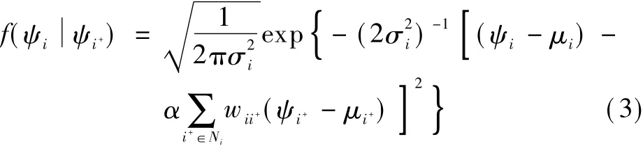
The joint probability density function is

whereEiis the exposure variable，which represents vehicle miles traveled(VMT)in this study;τ denotes an unknown parameter for the exposure measure;β0is the intercept term;βkdenotes the coefficient of thek-th covariate;Xikare indicators for thek-th covariate for segmenti;ψifollows the proper CAR prior，as described before;εiis a random error that has a gamma distribution，that is，εi～ Γ(θ，θ).

2 Data Description

In this study，roadways and crash data sets of Austin City in USA in 2010 are used to examine the associations between crash counts on mainlanes and the contributing factors.The roadways in this study are on-system highways， containing interstate highways， US highways，state highways，farm-to-market roadways，etc.In order to avoid the modifiable areal unit problem(MAUP)［19］，roadways are split into 1 824 homogeneous segments where geometric characteristics are coincident，as shown in Fig.1.Most segments have a length of 0 to 1.6 km and occupy more than 90%of the whole sample.The average of the segment length on mainlanes is 0.459 km.After merging crashes and segments，1 413 crashes on mainlanes are matched.

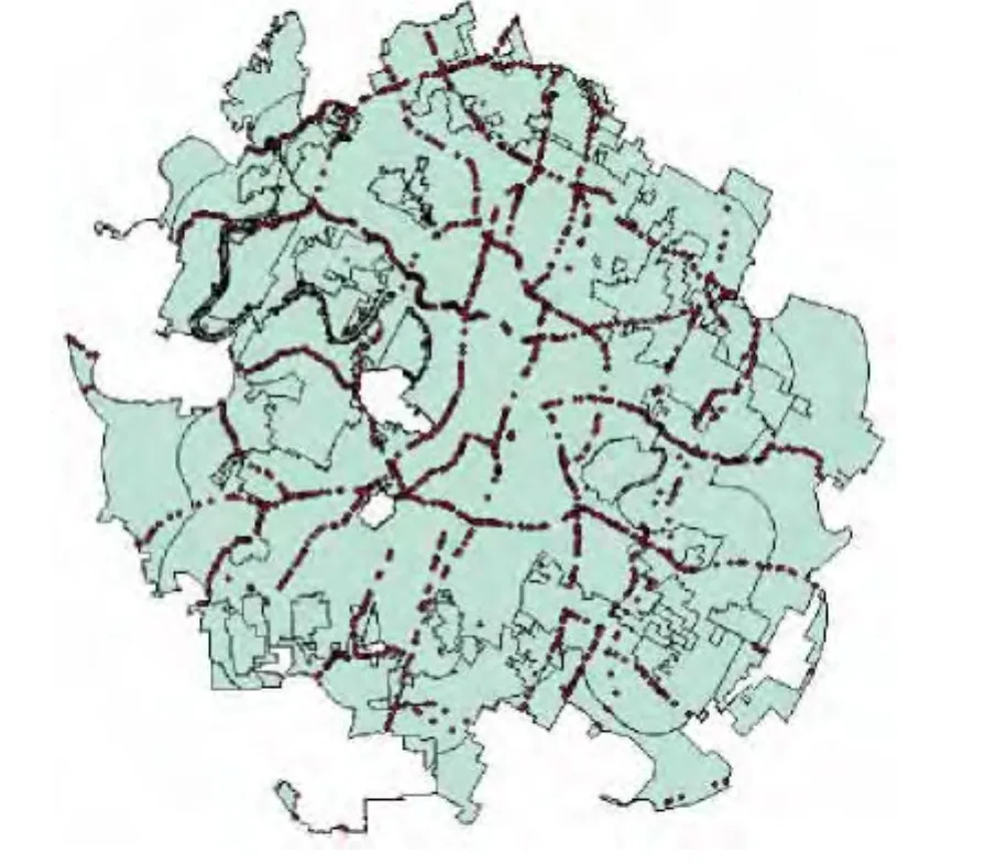
Fig.1 Distribution of homogeneous segments in Austin(Spots are the center points of segments)

In this study，the dependent variable is the number of crashes，while the exposure variable captures VMT，which is a key crash exposure term(since crash counts closely correlate with VMT，everything else remaining constant)，and simply the product of AADT，segment length，and 365 days per year.The dependent variable set contains both continuous and categorical variables，as shown in Tab.1.The indicator for curvature is a dummy variable，that is，if the answer is yes，it equals 1，and 0 otherwise.In addition，traffic characteristics allow for AADT，speed limit，and the percentage of truck AADT.In the past research，environments，especially distances to the nearest hospitals，were rarely employed for the contributing factors to analyze the associations of crash counts.In this study，hospitals are collected for analysis;meanwhile，the distances of which to segments are computed by ArcGIS，as shown in Fig.2.The data of annual rainfall obtained from the US Natural Resources Information System are also collected for analysis.It is noted that it would be best to match the year 2010 crashes to the same year rainfall data，however such information is unavailable，and we cannot find out the data.According to theclimate history in Texas，the annual rainfall changed a little，so 1961—1990 average rainfall is used instead.Fig.3 depicts the distribution of the annual rainfall in Austin.

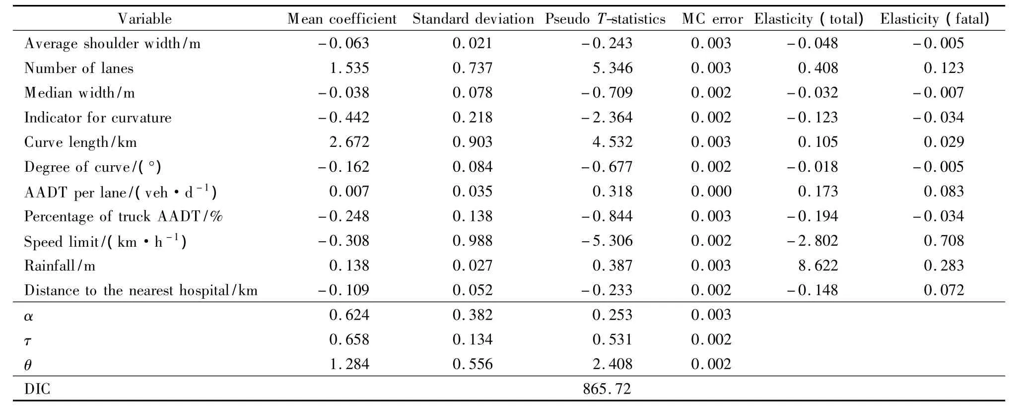
Tab.1 Summary statistics of variables for segments

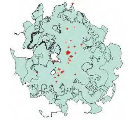
Fig.2 Distribution of hospitals in Austin

Fig.3 Distribution of annual rainfall in Austin

3 Estimation Results and Discussion

This section discusses the results of the associations between the contributing factors and the crash counts on mainlanes in Austin.Tab.2 shows the parameter estimates of the CAR model for crash counts，based on a total number of 5 000 draws in WinBUGS.

The association between crash exposure(VMT)and crash rates is estimated to be nonlinear(average exponent τ=0.658 for mainlanes)，which follows prior expectations.After controlling the exposure variable(VMT)，other covariates regardingcrash rates are estimated，which can be seen in Tab.2.

Elasticities for total crash counts and fatal crash counts are computed as the average percentage change in the mean crash rate per 1%change in thek-th variable.As shown in Tab.2，crash counts are estimated to have a statistically and practically significant spatial autocorrelation coefficient of 0.624(that is α =0.624).The number of lanes，curve length，AADT per lane，and rainfall have positive impacts on the mean crash rates for mainlanes，while the remaining variables all exhibit negative impacts on the mean crash rates.The elasticity of － 0.123 is found to be that of the curve indicator variables，implying that，holding everything else constant at their means，the mean crash rate is estimated to drop by 0.123 when the indicator variable switches from 0 to 1.The result confirms that the roadway curvature has negative effects on crash rates，which is consistent with the findings of some other studies［5-6］.

Interestingly，the speed limit on mainlanes exhibits negative mean elasticities，implying that higher speed limits are associated with lower mean crash rates，as found in Ref.［4］.However，the speed limit has a positive effect on fatality rates，as shown in Tab.2.Rainfall intensity is estimated to be positively associated with crash rates，and an increase of 1%rainfall will result in an increase of 8.622 in crash rates and an increase of 0.283 in fatality rates.As discussed previously，the distances to hospitals rarely appear as contributing factors in the crash modeling literature.It is found that the distances to the nearest hospitals have a negative impact on the mean crash rates，which suggests that shorter distances lead to higher crash rates，however，as expected，positive associations with fatal crash rates(presumably due to more severe collision impacts at higher speeds and time lost in transporting crash victims to an emergency room).

Tab.2 Estimation results of CAR-NB model for crash and fatal counts

In this study，the CAR-NB model is compared with another spatial model(CAR-Poisson)and some aspatial models(NB，zero-inflated NB and zero-inflated Poisson)，as shown in Tab.3.

Tab.3 Comparison of results using aspatial models and spatial models

The deviance information criterion(DIC)，as a generalization of the Akaike information criterion(AIC)，can be used to compare the goodness-of-fit and complexity of different models estimated under a Bayesian framework.The DIC equation is

whereD(θ¯)is the deviance evaluated atθ¯ which is the posterior mean of the parameters;pDis the effective number of parameters in the model;D¯ is the posterior mean of the deviance statisticD(θ).With regards to the model superiority and complexity，the lower the DIC，the better the model［20］.Tab.3 also presents the log likelihood values，which are used in the likelihood ratio chi-square to test whether all predictors'regression coefficients in the model are simultaneously zero.Meanwhile，Moran'sIis also considered，which is a measure of spatial autocorrelation developed by Moran［21］.Negative(positive)values indicate negative(positive)spatial autocorrelation and the values range from －1(indicating perfect dispersion)to+1(perfect correlation).

It is observed that the CAR-NB model has the lowest DIC and Moran'sIof residuals among these tested models.Meanwhile，mean log likelihood values of the CARNB model are the largest.The statistical tests suggest that the CAR-NB model is preferred over the CAR-Poisson，NB，zero-inflated Poisson，zero-inflated NB models due to its lower prediction errors and more robust parameter inference.It can be found that the negative binomial models in Tab.3 are better than the Poisson models due to the fact that overdispersion actually exists in the data.

4 Conclusions

1)Statistical tests of DIC，log likelihood and Moran'sIsuggest that the CAR-NB model is preferred over the CAR-Poisson，NB，zero-inflated Poisson，zero-inflated NB models，while the negative binomial models are better than the Poisson models.

2)The association between crash exposure(VMT)and crash rates is estimated to be nonlinear(average exponent τ =0.658 for mainlanes)，with crash rates effectively falling as VMT rises.

3)The number of lanes，curve length，AADT per lane，and rainfall have positive impacts on crash count，while the remaining variables all exhibit negative impacts.

4)The distances to the nearest hospitals and the speed limit have negative associations with segment-based crash counts but positive associations with fatality counts，presumably as a result of time loss during transporting crash victims and worsened collision impacts at higher speeds.

［1］Traffic Management Bureau of the Ministry of Public Security of the People's Republic of China.Road traffic accident statistics annual report of the People's Republic of China(2010)［R］.Wuxi:Traffic Management Research Institute of the Ministry of Public Security，2011.(in Chinese)

［2］Qu X，Guo T，Wang W，et al.Measuring speed consistency for freeway diverge areas using factor analysis［J］.Journal of Central South University:Science and Technology，2013，20(1):837-840.(in Chinese)

［3］Pei Y L，Ma J.Research on countermeasures for road condition causes of traffic accidents［J］.China Journal of Highway and Transport，2003，16(4):77-82.

［4］Ma J，Kockelman K M，Damien P.A multivariate Poisson-lognormal regression model for prediction of crash counts by severity，using Bayesian methods［J］.Accident Analysis and Prevention，2008，40(3):964-975.

［5］Quddus M A，Wang C，Ison S G.Road traffic congestion and crash severity:econometric analysis using ordered response models［J］.Journal of Transportation Engineering，2010，136(5):424-435.

［6］Wang C，Quddus M A，Ison S G.Predicting accident frequency at their severity levels and its application in site ranking using a two-stage mixed multivariate model［J］.Accident Analysis and Prevention，2011，43(6):1979-1990.

［7］Jovanis P，Chang H L.Modeling the relationship of accidents to miles traveled［J］.Transportation Research Record，1986，1068:42-51.

［8］Lord D.The prediction of accidents on digital networks:characteristics and issues related to the application of accident prediction models［D］.Toronto:University of Toronto，2000.

［9］Li L，Zhu L，Daniel Z S.A GIS-based Bayesian approach for analyzing spatial-temporal patterns of intra-city motor vehicle crashes［J］.Journal of Transport Geography，2007，15(4):274-285.

［10］Park B J，Lord D.Application of finite mixture models for vehicle crash data analysis［J］.Accident Analysis and Prevention，2009，41(4):683-91.

［11］Qin X，Reyes P.Conditional quantile analysis for crash count data［J］.Journal of Transportation Engineering，2011，137(9):601-607.

［12］Besag J E.Nearest-neighbour systems and the auto-logistic model for binary data［J］.Journal of the Royal Statistical Society，Series B:Methodological，1972，34(1):75-83.

［13］LeSage J P.Spatial econometrics［EB/OL］.(1999)［2013-03-15］.http://www.spatial-econometrics.com/.

［14］Miaou S，Song J J，Malick B.Roadway traffic crash mapping:a space-time modeling approach［J］.Journal of Transportation and Statistics，2003，6(1):33-57.

［15］Quddus M A.Modeling area-wide count outcomes with spatial correlation and heterogeneity:an analysis of London crash data［J］.Accident Analysis and Prevention，2008，40(4):1486-1497.

［16］Wang Y，Kockelman K M.A conditional-autoregressive count model for pedestrian crashes across neighborhoods［C/CD］//The92nd Annual Meeting of the Transportation Research Board.Washington DC，USA，2013.

［17］Anselin L.Spatial econometrics:methods and models［M］.Dordrecht:Kluwer Academic Publishers，1988.

［18］Mariella L，Tarantino M.Spatial temporal conditional auto-regressive model:a new autoregressive matrix ［J］.Australian Journal of Statistics，2010，39(3):223-244.

［19］Openshaw S.The modifiable areal unit problem ［J］.Concepts and Techniques in Modern Geography，1983，38:39-41.

［20］Spregelhalter D J，Best N G，Carlin B P，et al.Bayesian measures of model complexity and fit［J］.Journal of the Royal Statistical Society，Series B:Statistical Methodology，2002，64(4):583-639.

［21］Moran P A P.Notes on continuous stochastic phenomena［J］.Biometrika，1950，37(1):17-23.