Medical image segmentation based on neural network
2014-09-12WEIFeiLIUShoupeng
WEI Fei, LIU Shou-peng
(School of Health Management, Binzhou Medical University,Yantai 264003, China)
0 Introduction
The rapid development in the field of medical imaging has greatly promoted the progress of modern medicine. At present, computed tomography (CT), magnetic resonance imaging (MRI), ultrasound and other medical imaging technology has been widely used in clinical diagnosis and treatment. Segmentation is the basis for subsequent processing and three-dimensional visualization, surgical simulation and ultimate identification of diseased tissues. The accuracy of segmentation is crucial in correctly diagnosing patient’s condition; therefore image segmentation plays an important role in the field of medicine[1].
1 The structure of neural network for image segmentation
1.1 Back propagation neural network[2]
Back propagation learning algorithm, or BP algorithm, was introduced by D.E.Rumelhard and W.S.McClelland in 1986.Back propagation neural network is a supervised learning model. It composes of feed-forward networks and backward propagation of errors, and is the most popular neural network modeling tool. Back propagation neural network method is able to derive the underlying data relationship via an arbitrary set of input data. The key to this learning algorithm is via steepest descent, in which the algorithm automatically adjusts its network weight and threshold in order to minimize network delta. Back propagation neural network’s topology consists of input, hidden layer and output layer.
1.2 Parameter setting
Let’s assume there are 2 layers of neural network, the corresponding value of its input, hidden layer and output layers areX,n,y.
1) Number of neurons in input layer:X
The role of the neural network is equivalent to threshold method, ie, if a given input is greater than the threshold, it will be in the foreground, else it goes to the background. Its value is the actual input vectorX=(x1,x2,…,xn)T.
2) Number of neurons in output layer:y
Node in this layer represents the output variable. In a multi-input, single-output system, the number of nodes in the layer defaults to 1, the initial value iswiunder rough membership function degree value. The output of this layer node
(1)
3) Number of neurons in hidden layer:n
Dividennumber of input(x1,x2,…,xn)into different categories randomly. Assign a weight to reach input, the weight is to be between the value of [0,1]. Define the neuronal function of this layer as Gauss function
(2)
where,i=1,2,…,n,j=1,2,…,r,ras a discrete number of segmentation,mijas the center of the mean,σijdecided to its width.
4) Each layer activation function
Each layer of nodes representing a rule, assuming there arek(k≤n) rule, the layer nodes action functions as
(3)
Fig.1 is the structure of neural network.

Fig.1 The structure of neural network
2 Optimization
Taking into account that the nature of neural networks is an m-dimensional input vectorsX=(X1,…,Xm) transformation to theq-dimensional output vectorsO=(O1,…,Oq) is the non-linear mapping[3]. During experiment, given an input sample vector, its output is the actual weight and set over’s independent variable function
a=F(W,b),
(4)
where,Wandbare the weight matrix and set over the matrix,ais the actual output of the network.
Assumetis the corresponding desired output,SNis the total number of sample, then the minimal mean square deviation can be expressed as (MSE is mean square error)
(5)
Constantly adjust the weights between nodes and set over, the result will eventually approximate the desired output.
Relying purely on the network’s own algorithm to achieve network convergence tends to lead to local optimization. Therefore particle swarm optimization algorithm is used and implemented as shon in Fig.2 of the 3 mappings[4].

Particle swarm optimization Neural Network
Fig.2Mappingbetweenneuralnetworkandparticleswarmoptimization
1) Mapping between neural network’s weights and particle dimension space
Dimension of each particle in the particle swarm corresponds to a weight in the neural network. Vice versa, the weight and set over in the neural network equal to each particle in the particle swarm optimization.
2) Mapping between neural network MSE and particle swarm optimization fitness function
MSE of the neural network is a particle swarm optimization fitness function. It should be minimized via the powerful search performance provided by particle swarm optimization.
3) Neural network learning and particle search
The learning process of neural network is about continuously updating the weight and delta to minimize the MSE. The search process of particle swarm optimization is the dimensional change of speed and position of the particles. Taking into account that each particle corresponds to a neural network’s weight and set over, neural network learning process is equivalent to the search for the most optimal location of particles.
3 Image segmentation
3.1 Image area description
Image regional boundaries are represented via regional content and area boundaries. Regional content is often differentiated via colors, texture and geometric meoments, while the regional boundary’s often differentiated by circular degree, rectangle degree etc.
Fig.3 depicted the multiple images in the simple region. Image 2 is derived from image 1 through pan and zoom, image 4 is derived from image 2 via rotations and translations, while image 6 is derived from image 5 through rotation and scaling.

Fig.3 Image area
On the basis of a neural network as the classifier’s thoughts on the divided region, the image region matching into image area between matching, this can effectively reduce the complexity of image matching, improves the efficiency of the algorithm.
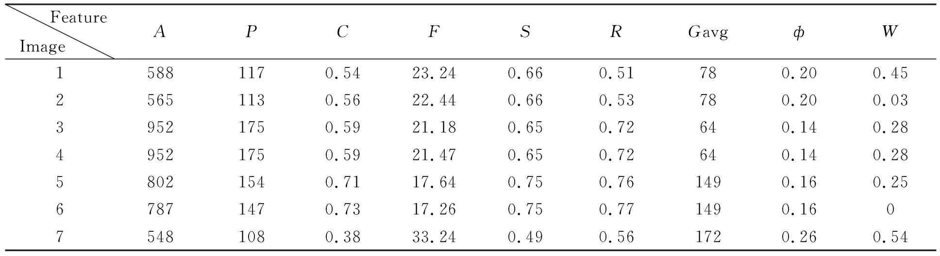
Extraction of regional characteristics and measurement results as shown in Tab.1.
Tab.1 Image region characteristic data sheet
Where,A: acreage,P:circumference,C: circularity,F: contour complexity,S: roundness,R: rectangularity,Gavg: gray level, ф: area moment,W: texture.
3.2 Data discretization
Based on the maximum and minimum truncation point discretization algorithm simply puts the data into 3 categories, does not require any type of information, the algorithm is as follows: maximum and minimum truncation point discretization algorithm.
Input:nsamples ofMfeature value data ( see Tab.1), the output: decision tableT=(U,C∪D,V,f).
Step 1 The attribute value setVa=(C0a,C1a,…,CKa) in increasing order ( the same attribute value to take only one ) and divided into interval equivalence classes. ∪[Cia,Ci+1a], whicha∈C∪D,0≤i Step 2 Using the midpoint method to find out the interval [Cia,Ci+1a] truncatedCicomposed of truncated point setVa=(C0,C1,…,CK-1). Step 3 Minimum and maximum cut-off pointC0,CK-1. Step 4 Category tag. (6) For decision table, the tables in the same row are merged, to get Tab.2. In Tab.2, various features as condition attributes, add category as decision attribute. Tab.2 Decision table UsingA.Skowrondiscernibilitymatrixmethodofdecisiontablereductionstep2,asfollows: Step1CalculatethedecisionTab.2correspondingdiscernibilitymatrixM(C,D). Step2UsingthediscernibilitymatrixpropertiesthatattributeSisnuclear,deletethediscernibilitymatrixM(C,D)allcontaintheattributeSitem. Step3CalculationofthenumberofoccurrencesofeachattributeNA=NP=NG=Nφ=2, NR=1,sothereductionofattributesset{S,φ}and{S, G}. Asaresultofdecisiontablereduction,thispaperchooses{S,φ}.Theintuitivemeaningisthroughtheimageareaofthesphericalandregionalmomentinvariantfeaturesofdifferenceimagearea. Accordingtotheobtainedreduction,Tab.2canbesimplifiedtoTab.3,inthesamebankmerger. Tab.3 The depicted multiple images in the simple region WhenAis an equivalence relation between objects in the domainU, thenU/Arepresents all equivalence classes of objects based on family relationshipUAcomposition. The decision rules are as follows: Rule of 1:S1ф1→Class1, Rule of 2:S1ф0→Class2, Rule of 3:S2ф1→Class3, Rule of 4:S0ф2→Class4. Apparently consistent decision table, for each of which a regulation is consistent. Corresponding neural network model based on the above data processing methods, that is: the number of nodes in the first layer-4, the number of nodes in the second layer-4, the number of nodes in the third layer-4, fourth layer nodes is 1. The initial value of the connection weights between the third layer and fourth layer should be set as membership function degree value. Input of each neuron unit is the regional value, apply back propagation algorithm iterations, the output values are candidates for final decision results. Image segmentation is achieved through polymerization. Divide the 86 medical images collected from Internet into two categories. For the first category, manually segment the image using photoshop to achieve most optimal result, and this will be used as the sample input for neural network. The second category is the test sample[6-11]. The initial structure of the neural network is set to 9-20-1, and then use the methods described in 3.3 to build the decision tree as shown in Fig.4. By looking at the decision tree, we eventually found seven major nodes {1,2,4,6,7,11,18}, therefore, the network results eventually identified as 9-7-1. Fig.4 The decision tree is used to determine the number of neurons in hidden layer (6) (7) (8) Among them,ηfor the learning rate,βfor the modified step coefficient,αfor inertia coefficient(0≤α≤1). The use of matlab language programming neural networkimage segmentation. The following image segmentation is shown in Fig.5. (a)Original image (b) Segmented image Fig.5(a) is the original image. Figure in the two larger cells are white blood cells, and the rest are small red blood cells. Fig.5 (b) shows the back propagation algorithm segmentation results. Experimental result indicates that segmentation provided a clearly image and highlight target area. This approach significantly reduces training time, improves accuracy, and is superior to conventional segmented images when it comes to meet real-time medical image processing requirements. It presented a whole new set of ideas that’s very effective. This paper presents back propagation neural network based image segmentation approach. The experiments show that this method greatly reducing the training time and improve the accuracy, but will also be superior to conventional image segmentation, image processing to meet the real-time requirements. The method has great potential in the field of image segmentation, and its impact is still to be further investigated. : [1] Pawlak Z. Rough sets[J].International Journal of Information and Computer Science,1982,11:341-256. [2] Liu Q. Rough set and rough reasoning[M].Beijing:Science Press,2001. [3] Zeng H L. Rough set theory and its application[M].Chongqing: Chongqing University Press,1998. [4] Zeng H L, Zeng Q. The neural network based on rough set theory[J].Journal of Sichuan College of Chemical Light,2000,13(1):1-5. [5] Xu Z X, Ding Y L. A method based on rough neural networks of rough set theory[J].Nanjing University of Aeronautics and Astronautics Journal,2001,33(4):355-358. [6] Li N Y. Rough set theory and its application in image segmentation[J].Sanming Journal,2005,22(4):382-385. [7] Jelonek J. Rough set reduction of attributes and their domains for neural net-works[J].Computational Intelligence, 1995,11(2):339-347. [8] Zhang Y D, Wu L N. Optimizing weights of neural network using BCO[J].PIER,2008,83:185-198. [9] Zhang Y D, Wu L N. A novel pattern recognition method via PCNN and tsallis entropy[J].Sensors,2008,8(11):7518-7529. [10] Lin X M, Lv S S, Zhu D, et al. A new particle swarm optimization algorithm for medical image segmentation based on neural network[J].Journal of Changchun University of Technology: Nature Science Edition,2008,29(2):158-161. [11] Hong W C. Chaotic particle swarm optimization algorithm in a support vector regression electric load forecasting model[J].Energy Conversion and Management,2009,50:105-117.
3.3 Attribute reduction[5]
3.4 Rule acquisition

3.5 Principle
4 Experimental results and analysis
4.1 Experimental procedure

4.2 Network experimental result

5 Conclusions