Water flooding optimization with adjoint model under control constraints*
2014-06-01ZHANGKai张凯ZHANGLiming张黎明YAOJun姚军CHENYuxue陈玉雪
ZHANG Kai (张凯), ZHANG Li-ming (张黎明), YAO Jun (姚军), CHEN Yu-xue (陈玉雪),
LU Ran-ran (路然然)
School of Petroleum Engineering, China University of Petroleum (East China), Qingdao 266580, China, E-mail: reservoirs@163.com
Water flooding optimization with adjoint model under control constraints*
ZHANG Kai (张凯), ZHANG Li-ming (张黎明), YAO Jun (姚军), CHEN Yu-xue (陈玉雪),
LU Ran-ran (路然然)
School of Petroleum Engineering, China University of Petroleum (East China), Qingdao 266580, China, E-mail: reservoirs@163.com
(Received November 16, 2012, Revised March 8, 2013)
The oil recovery enhancement is a major technical issue in the development of oil and gas fields. The smart oil field is an effective way to deal with the issue. It can achieve the maximum profits in the oil production at a minimum cost, and represents the future direction of oil fields. This paper discusses the core of the smart field theory, mainly the real-time optimization method of the injection-production rate of water-oil wells in a complex oil-gas filtration system. Computing speed is considered as the primary prerequisite because this research depends very much on reservoir numerical simulations and each simulation may take several hours or even days. An adjoint gradient method of the maximum theory is chosen for the solution of the optimal control variables. Conventional solving method of the maximum principle requires two solutions of time series: the forward reservoir simulation and the backward adjoint gradient calculation. In this paper, the two processes are combined together and a fully implicit reservoir simulator is developed. The matrixes of the adjoint equation are directly obtained from the fully implicit reservoir simulation, which accelerates the optimization solution and enhances the efficiency of the solving model. Meanwhile, a gradient projection algorithm combined with the maximum theory is used to constrain the parameters in the oil field development, which make it possible for the method to be applied to the water flooding optimization in a real oil field. The above theory is tested in several reservoir cases and it is shown that a better development effect of the oil field can be achieved.
water flooding optimization, adjoint model, fully implicit simulation, constrained optimization, gradient projection
Introduction
As is well known, almost all reservoirs are heterogeneous and the injection water would rapidly break through along high-permeability channels to production wells. Therefore, the water can not drive the oil like a piston, along uneven waterlines. The conventional way is to design orthogonal experiments for different production plans to determine a reasonable start time of water flooding and the production/injection rate. However, all these different production parameters are set by hand, and the results are heavily affected by subjective factors. As a result, the chosen plan might not be the optimal one for a given reservoir. Meanwhile, the process will take a considerable amount of time and labour and is not feasible enough to determine the real-time production adjustment plan.
In 2004, Brouwer[1]et al., Delft University of Technology, The Netherlands, proposed a new forecasting method, for the reservoir production optimal control, which combines the reservoir numerical simulation with the optimization theory. It can be used to adjust the performance of the reservoir and to obtain the optimal control rates to maximize economic profits. The main parameters to optimize include: the production rate, the injection rate and the bottomhole flowing pressure. The final objective of the optimal control is to provide the best real-time production plan in a rapid and convenient way.
To solve the mathematical model of the optimal control for the reservoir development, there are mainly two kinds of methods as follows:
(1) Gradient-based algorithms. Wang et al.[2]used the perturbation method to calculate the gradientof the optimal control model. The calculation of the gradient is simple but time-consuming, and each perturbation requires two reservoir simulations at least. Brouwer[1], Jansen et al.[3]and Zhang et al.[4]calculated the gradient of the model using the maximum principle. But they do not combine the two processes together and constrain the injection-production parameters. Chen et al.[5]proposed an augmented Lagrangian method for the production optimization and a way to avoid the need to convert the inequality constraints to equality constraints. Zhang et al.[6]optimized well placement and production together using gradient algorithm. Jansen[7]discussed in detail various aspects of the adjoint-based optimization of the reservoir fooding including the optimal control theory, the computational aspects and the operational use. Although the gradient-based algorithms make the fastest calculations, they are more complex than other methods and it is difficult to develop related programs.
(2) Stochastic algorithms. Alghareeb et al.[8]and Chen et al.[9]used the genetic algorithm to optimize the injection and production strategy to find a global optimal solution through large-scale computing, but this method has a low efficiency as a result of too many iterations. Lorentzen et al.[10], Chaudhri et al.[11], Chen and Oliver[12]used the Ensemble Kalman filter (EnKF) as well as its improved methods EnOpt to complete the production optimization. Shuai et al.[13]applied the multiscale regularization to EnOpt and to the bound optimization by quadratic approximation (BOBYQA) to address the problem brought by too high or too low frequencies in the control adjustment. With the multiscale regularization, both methods can be used to obtain the net value of production (NVP) that is equal to or exceeds the unregularized optimization, with simpler well control strategies and to reach a convergence in fewer iterations. Chen[14]tested three derivative-free algorithms: VFSA, SPMI and QIM, all in good matches and verified the fact that the DFO algorithm is capable and applicable in simulators without an adjoint formulation built in. Zhao et al.[15]proposed a new derivative-free optimization algorithm (QIM-AG) for the production optimization. Although this algorithm performs better in terms of the value of NPV attained and the computational efficiency than other derivative-free algorithms tested, it still requires more simulation runs and with a lower NPV than the adjoint-based method. And in the same year, Yan and Reynolds[16]developed a more robust optimization procedure and presented several versions of SGFD-based search direction methods that combine the fnite difference approximations with the stochastic gradients.
A great number of reservoir numerical simulations are required in this kind of study and each simulation may take several hours or even days, therefore, for the field applications of the water flooding optimization, the computing speed is an essential issue. So the gradient algorithm is chosen as our research method.
1. The optimal control of reservoir development
The objective of the optimal control is to let the reservoir development system reach its best working states by an optimal plan. A mathematical model of the development optimization is to be built. Because the produced amounts of oil and water are calculated by the reservoir simulator, the flow equations of each grid block in the reservoir simulation should be considered in the model. They are expressed as follows:
The specific parameters in this model are as follows:
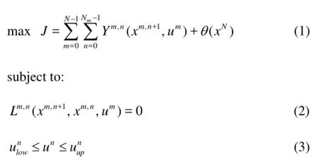
(1)Jthe objective function, consists of two components, the performance indicator of the optimal control strategy,mnY(NPV) and the additional cost of expensesθ(e.g., the cost of depreciation). In this paper,Ym,nis the increment ofJduring the thnsampling period. In the reservoir production optimization,Ym,nis composed of variables like the flow rate or the function of saturation (sweep efficiency), and its specific expression is as follows

where,ojQis the oil production rate of the thjlayer per time interval for a single well.,wjQis the water production rate of the thjlayer per time interval for a single well. ,wi jQis the injection rate of the thjlayer per time interval for a single well.oris the economical factor of the crude output.wpris the prime cost factor of the water production.wiris the prime cost factor of the water injection.tΔ is the time interval, year.bis the current interest rate.PNis the number of producing wells.INis the number of injectionwells.mis the simulation time step in each control time step.
(2)Ltogether with the initial condition makes up the reservoir dynamic system consisting of a number of equations of the fully implicit 3-D, 3-phase black oil model (see Eq.(16)).
(3) Equation (3) are the boundary constraints of the control variables. Other inequality constraints can also be added if, for example, the field oil production rate cannot be above the field operation limits or the economic limit cannot be higher than the Water-Oil-Ratio.
(4)xis a dynamic variable (e.g., the pressure, the saturation, the component.).uis a control variable (the flow rate of the production or injection well).Nis the total number of control time steps.mNis the total number of simulating time steps in each control step.
The problem can be described as follows: to achieve an optimal control strategy ()u t*and the corresponding optimal statex*for the objective functionJto take the maximum and on condition that the control variables satisfy the linear constraints Eq.(3) (e.g., the extreme value of a single well).
2. Optimal control solution
2.1Discrete maximum principle
The maximum principle is a method based on the variational theory. It is a theoretical foundation of the optimal control theory and can be applied to solve reservoir production problems. Firstly, we construct the Lagrange function with Eq.(1) and Eq.(2).

According to the maximum principle, the first order variation ofAJis

By using the principle of integration by parts,

In order to obtain the maximum ofAJ,AJδmust be equal to 0, which means that every item in Eq.(8) must be equal to 0. These items will be analyzed in the following manner
(1) Adjoint equation (1st item of Eq.(8))
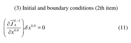
The data for the initial reservoir conditions like those on the oil-water contact surface can be measured. So the initial reservoir pressure and saturation distributions of state variables (x0,0) are known. Therefore,δx0,0=0, which means that the condition Eq.(11) is automatically satisfied too.
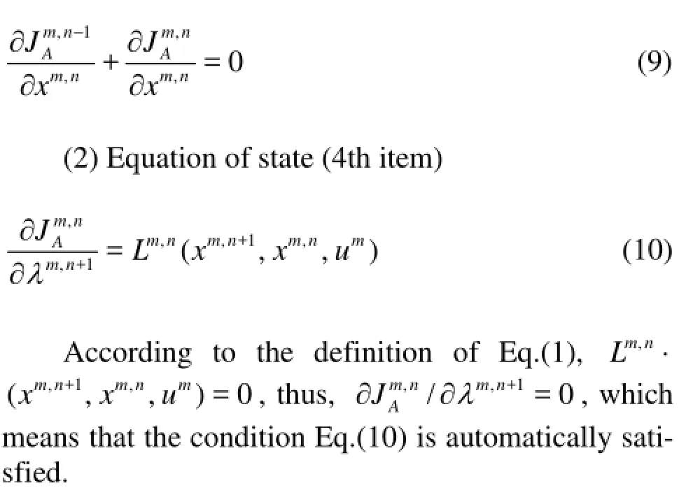
(4) Last boundary condition (3th item)

The conditions of (2) and (3) are satisfied automatically. According to (1) and (4) we can establish the adjoint model.
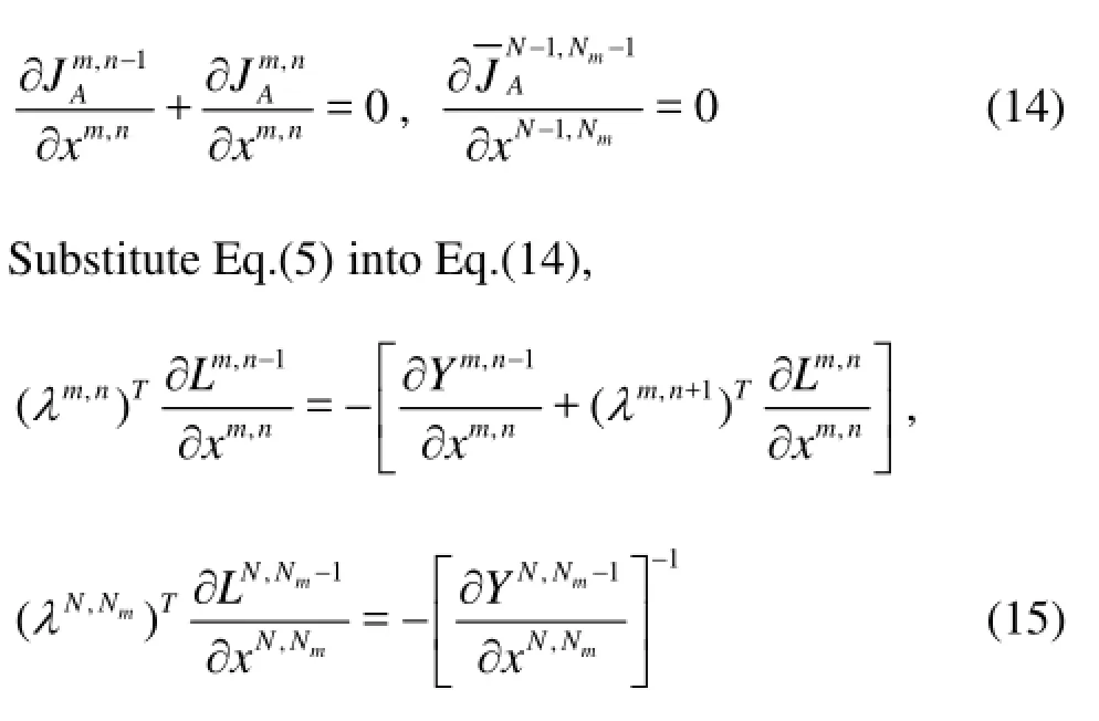
Theλcan be obtained by solving the adjoint model Eq.(15) backward from theNth to 1st step. and with its being substituted into Eq.(13), the gradient ∇JAand the control variables can be calculated. And then the objective function is evaluated by these control variables. If ∇JAis not equal to 0, these processes will be repeated. When it is equal to 0, the optimal control plan is achieved.
2.2Calculation of variables
According to the aforementioned method, two solutions of time series are required and are to be obtained by the forward reservoir simulation and the backward adjoint gradient calculation. Given the characteristics of the adjoint and gradient equations, a total of 4 terms need to be solved, namely ∂Y/∂x,∂Y/∂u, ∂L/∂xand ∂L/∂u.

Fig.1 Mesh diagram
2.2.1 Calculation of /Lx∂∂
The solving process of the gradient mentioned above is based on the maximum principle and the reservoir numerical simulation. The reservoir simulation is mainly used to simulate the whole process of the oil reservoir development in a numerical way and it involves the calculations of the flows of the oil, the water and the gas, due to the unbalanced pressures in the heterogeneous reservoir. Therefore, the reservoir is meshed and the pressure in each grid block needs to be solved. The basic pressure equation of the fully implicit black oil model in the reservoir simulator is

whereLis the pressure equation of the fully implicit black oil model,ηis the accumulated items of the mass conservation equation,ψis the flux item of the mass conservation equation,Wis the flow rate of the production or injection well,Vis the volume,φis the porosity,Spis the saturation,ρpis the density,Xcpis the moles of the componentcin the phasep, Δtis the time interval,Tsis the conductivity,λpis the mobility of phasep, ΔΦpis the potential difference of the phasep,nis the time step,Ppis the grid pressure, andPwfis the bottomhole flowing pressure.
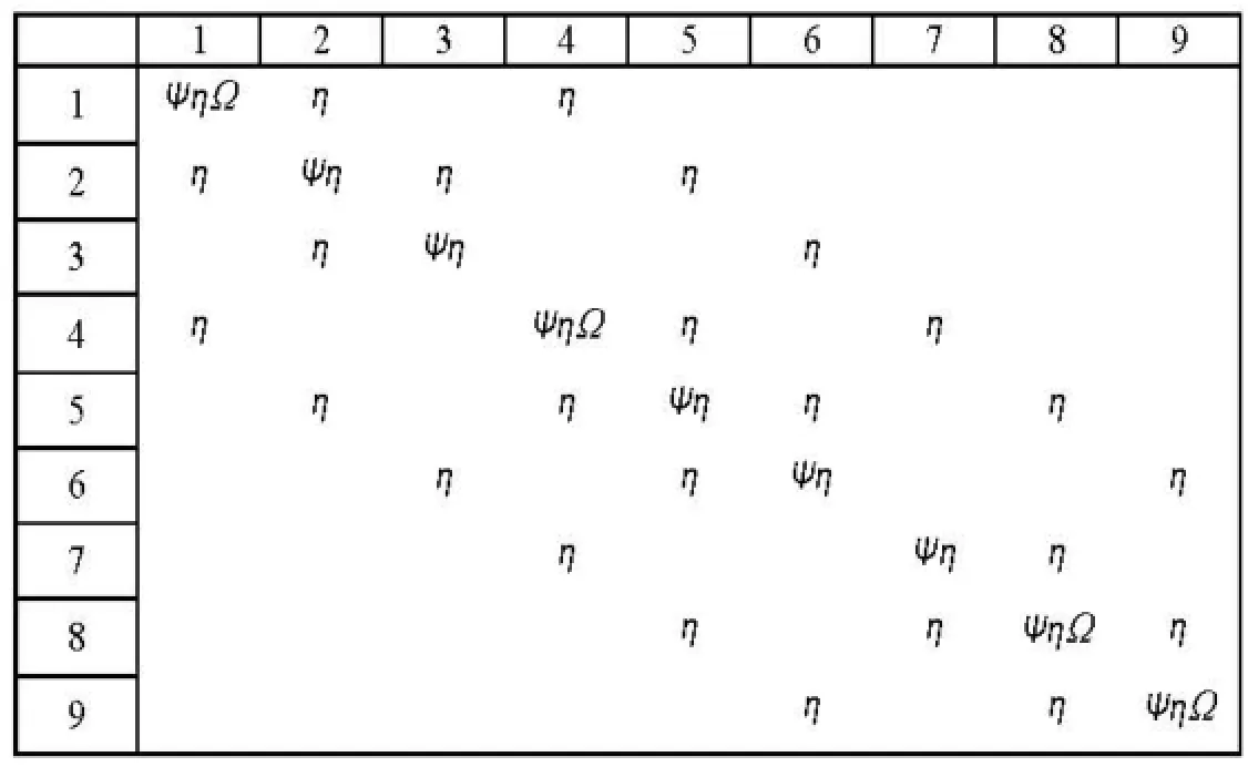
Fig.2 Jacobian matrix
The Jacobian matrix, containing all information for the whole reservoir, is rather huge and we will just consider a small case of 3×3 model as an example (as shown in Fig.1). There are two wells in the reservoir, one is perforated at grid 1 and grid 4, and the other at grid 8 and grid 9. The Jacobian matrix is obtained from Eq.(16), as shown in Fig.2. It is a pentadiagonal matrix and with different linearization methods, different matrices are obtained. For example, if the Newton-Raphson method is adopted, all items in the matrix should be changed into the partial derivatives of the state variables. For an easy understanding, the grid (1,1) will be taken as an example, as it contains partsA,FandWin Eq.(16). There are three phases, including the oil, the gas and the water, in the reservoir, so each grid has three independent variables for the three-phase flow equations. The partial derivatives of the three flow equations with respect to the three control variables are as follows

wheregLis the gas flow equation,oLis the oil flow equation,wLis the water flow equation,gPis the gas pressure,gSis the gas saturation, andoSis the oil saturation.
So the Jacobian matrix of the fully implicit reservoir simulation can be expressed as follows

According to Eq.(16), ∂Lm,n/∂xm,nin model (16) should be

In this case, ∂ηm,n(xm,n)/∂xm,ncan be obtained at the previous time stepn-1, which means that it is not necessary to calculate this term at thenth step and the previous result ∂Lm,n/∂xm,ncan be extracted directly.
2.2.2 Calculation of /Yx∂∂, /Yu∂∂ and /Lu∂∂
We ignore the effect of the density on the change of state variables when taking derivatives with respect toxand the derivative can be expressed as follows

where /Wx∂∂ is just a part of /Lx∂∂ which can be obtained directly from the Jacobian matrix by the fully implicit solution. The dimension of /Yx∂∂ is 1Ne×. As for /Yu∂∂ and /Lu∂∂, they can be calculated in the process of the numerical simulation. The results of each time step are kept and then used directly in the follow-up backward gradient calculations.
3. Constrained optimization
The numerical reservoir simulation is a large-scale computation, involving also many constraints, related with such as the extreme values for production (WOPR) or the injection rate (WWIR) of a single well, the maximum field total production (FOPT) and injection (FWIT) rates, the field highest water cut(FWCT). Therefore, the water flooding optimization is always a rather complicated constrained optimal control.
3.1Advantages of gradient projection
(1) Only one adjoint gradient is needed using the maximal principle for each iteration.
(2) During the whole optimization process, all solutions are feasible. And a large step size can be used to accelerate the optimization.
Compared with the feasible direction method proposed by Sarma[17], this method is more suitable for the reservoir simulation with a simpler computation process, a faster speed and better outcomes.
3.2Gradient projection algorithm
The gradient projection algorithm is the natural extension of the steepest descent algorithm for bound constrained problems. The constrained problem is defined as

whereAis a matrix composed ofam,uis the con-
原文:http://www.dpm.org.cn/collection/ceramic/226720.html?hl=%E8%B1%A1%E8%80%B3%E8%BD%AC%E5%BF%83%E7%93%B6
Pitrol variables as above mentioned (the flow rate oil production or the injection well per day),bis the total production or injection rate per day. These equations determine the lower limit of the total production and injection rate per day in a reservoir. With the results, the optimization process could maintain the formation energy and ensure the balance of the production and the injection

Fig.3 Search sketch of projected gradient method
The gradient projection method is used to solve the model. The basic assumption of the method is thatulies in the subspace tangent to the active constraints. If the iterative downhill search+1lgbreaches the constraint conditions, the search is to be changed along the projected gradient direction+1ld(as shown in Fig.3), wherelis the iteration step.
In the process of the iterative uphill search, the new variables can be updated by

where+1lαcan be obtained by the line search. Using Eq.(24) in Eq.(26),

Comparing Eq.(21) with Eq.(22), it follows that the linear constraints can only be satisfied by requiring that

In order to obtain the maximum NPV, it is hoped thatdl+1deviates from thegl+1as small as possible. Therefore, the new mathematical model constrained by Eq.(21) can be constructed as


The projected gradient can be calculated by Eq.(30). P is called the projection matrix. After a search direction is determined, a one dimensional search must be carried out to determine the value ofαin Eq.(22).
4. Procedure of optimal calculation
(1) With the initial conditions and the working systems, the reservoir model is solved along the forward time-scale, ∂W/∂xand ∂W/∂u, as well as the Jacobian matrix are saved for each time step.
(2) The adjoint equation is solved along the reverse time-scale by the maximum principle. With the reserved matrix for each time step, we can obtain the variables (∂Y/∂x, ∂Y/∂u, ∂L/∂xand ∂L/∂u) directly, then calculate the Lagrange multiplier for each time step.
(3) With the Lagrange multiplier, the gradient∂JA/∂uis calculated corresponding to all control variables by Eq.(13).

(5) The gradient projection algorithm is used to calculate the constrained gradient by Eq.(30).
(6) On the basis of the gradient, we can reach a new set of the control variables by a linear search, then use the log-inverse transformation to obtain the optimized control variableu, thus design a new development plan.
(7) The optimization process is repeated until the gradients of all the control variables approach zero.
5. Case study
5.1Fully implicit simulator
Because the study mainly concerns the mixed solution of the simulator and the optimization algorithm, the preparation of the fully implicit reservoir simulator plays a key role. This implicit reservoir simulator is developed by our group, the classic SPE1 reservoir simulation model[18]is tested, and the results are compared with those of the commercial simulator Eclipse to verify the calculations made by the simulator.
For the two simulators, the same time steps, 32 steps are used, and the number of Newton iterations of the compiled simulator is 109. The comparisons of the results between the compiled simulator and Eclipse are shown in Figs.4 and 5. Figure 4 is a comparison of the daily oil production, from which we can see that a stable production occurs after about 1 000 d. The oil production goes from the constant oil production control to the bottomhole pressure control and the oil production is gradually decreased. Figure 5 shows the comparison of the producing gas oil ratio (GOR). At the initial state of the reservoir, there is no free gas, so the GOR is constant. About 660 d later, the free gas emerges and the GOR begins to increase steadily. In the comparison, the results of the simulator and Eclipse calculations are almost identical, which lays a good foundation for the subsequent optimization of the reservoir control.

Fig.4 Simulator results of daily oil production comparison

Fig.5 Simulator results of GOR comparison

Fig.6 Sketch map of two smart horizontal wells
5.2Optimization of reservoir examples
5.2.1 Theoretical model optimization
The waterflood optimization is carried out for a 2-D heterogeneous reservoir as shown in Figs.6-12. The model consists of one horizontal “smart” water injector and one horizontal “smart” producer, eachwith 45 controllable segments. The reservoir is 450 m2×450 m2in width and length and 10 m in thickness. It is modeled as 45×45×1. The fluid system is in essentially incompressible oil-water two phases, in 0.1 connate water saturation and 0.1 residual oil saturation. The initial reservoir pressure is 40 MPa. Figure 7 shows the heterogeneous permeability field with two high permeability channels running from the injector (left) to the producer (right).

Fig.7 Permeability field of theoretical model

Fig.8 NPV in the process of optimization

Fig.9 Comparison of accumulative oil and water before and after optimization
For the purpose of optimization, the injector segments are placed under the rate control, and the producer segments are placed under the pressure control. The total injection constraint rate of 368.68 m3/d is distributed in 45 injector segments according tokh. The overall production lasts about 950 d, and the production strategy changes every 190 days, which means that there are 5 control steps in the whole production life. Therefore the number of control variables can be calculated as (45+45)×5=450. And this model is designed to validate the discrete maximum principle method.
From our calculation experience, it can be justifiably concluded that the difference between the calculated gradient of a single well by the maximum theory and that by the perturbation is negligible.
With the projected gradient method, the constrained optimization of the total injection rate for every step can be realized. Distributing the water injection for each well while setting the total injection rate as a constant value, the effectiveness of the proposed optimization technique can be testified.
The oil price is conservatively set as 80$/bbl, the water production cost as 30$/bbl, and the water injection cost as 10$/bbl. Figure 9 shows that there is a 57.8% increase in the cumulative field oil production (FOPT) due to a better sweep, and an evident decrease in the field water production (FWPT) of 37.3% and a water cut (FWCT), leading to an increase of NPV from 1.7×10⁷$ to 8.45×10⁷$.
Figure 10(a) shows that the water floods quickly along the two high-permeability channels with a regular production strategy without optimization. As a result, a large scale oil is upswept in the comparatively low-permeability zone. And the low water sweep efficiency reduces the reservoir recovery rate. The well production schedule is changed every 190 d in the whole production life according to the optimization results after 22 iterations. The ultimate saturation field is shown in Fig.10(b). From the saturation distribution of the optimization strategy as compared with that of the regular production strategy, it can be seen that most of reservoir oil can be displaced by water, leaving little peripheral oil behind. Therefore, the recovery rate is increased significantly.
The reason behind the better sweep in the optimized case can be easily explained by analyzing the optimized trajectories of the controls-rates/BHPs of the injectors/producers, as shown in Figs.11 and 12. From Fig.11, it can be seen that the injection rates near high permeability channels are nearly zero in the first 190 d and increase gradually from the third control step. From Fig.13, it is seen that the BHPs are increased and the production rates are decreased near high permeability channels from the third control step, which can delay the water fingering caused by the injected water increase.

Fig.10 Oil saturation distribution optimization at 0 d, 190 d, 380 d, 540 d, 730 d and 950 d

Fig.11 Injection water rate distribution of injectors in different control steps

Fig.12 BHP distribution of producers in different control steps
5.2.2 Oil field applications
The aforementioned theory is applied to the 27A block in the Shengli Chengdao oilfield, to find an optimal development design. There are five wells in this area, two of which (A1 and A5) are production wells, two (A4 and A6) are injection wells, and the well A3 is shutdown. The three main layers in this block are Ng35, Ng36 and Ng45. To search for the optimal control of this reservoir, the flowing rate of each injectors and producers drilling through these three layers is treated as one control variable and will be distributed to each layer by the fully implicit reservoir simulator automatically. Thus for the same development design, different layers may have different recovery efficiencies. The production began in February 1998, and turned into the water flooding in March 2002. The well area is divided by the driving energy into the development stage of the natural energy (1998-2-2002-3), and the water injection development stage (2002-3-present).

Fig.13 Control map of the wells after optimization

Table 1 Comparison of recovery rate
Up to now, as shown in Table 1, the cumulative recovery ratio of the block has reached 15.75%. The digital-analog method is used to forecast 5-year production targets. During this time, the cumulative oil production is 49 600 t, and the recovery rate is 18.35%, While according to the aforementioned optimization control method, also forecasting five-year, with one control every six months and the optimiza-tion time is divided into 10 steps (0 d, 182 d, 365 d, 547 d, 730 d, 912 d, 1 095 d, 1 277 d, 1 460 d and 1 642 d). The initial bottom hole pressures of the production wells A1 and A5 are 10.15 MPa. The initial injection rates of A4 and A6 are 120 m3/d. The total injection rate is constrained to 240 m3/d. After optimization the recovery rate reaches 19.27%, an increase of 0.92% as compared with that before optimization. The cumulative increase of the oil production is 11 300 t, and the net present value is increased by 35%.

Fig.14 Water cut and accumulative production of oil and water before and after optimization
The accumulative field productions of the oil (FOPT) and the water (FWPT) before and after optimization are shown in Fig.14. We can see that after optimization, the water cut of the block is not increased noticeably. Although the FWPT increases, there is a greater increase in the accumulative production of the oil, reaching the target to increase the oil and to control the water.
With the constant total injection rate, the effect of increasing oil is caused by the injection increase of A4 from 120 m3/d to 240 m3/d (see Fig.13). With the injection of A6 being reduced to 0 m3/d, the sweep efficiency around A4 increases, as shown in Figs.15 and 16. The injection water fingering phenomena of A6 are decreased and more oil is produced in Ng35 and Ng45 formations.

Fig.15 Final oil saturation distribution of the reference case
6. Conclusions
(1) A reservoir development control optimization model is established and solved by the maximum principle method. The solved adjoint gradients are verified with a comparison with the perturbation gradients.
(2) All iterations are feasible states, implying that the optimization may be stopped at any iteration and the final iteration can be considered a useful solution.
(3) The projected gradient algorithm can be effectively used to constrain the FOPT, the FWIT and other parameters. While large step sizes are possible during the modified line search, a significant reduction of the objective function may be resulted by these constrained conditions.
[1] BROUWER D. R. Dynamic water flood optimization with smart wells using optimal control theory[D]. Delft, The Netherlands: Delft University of Technology, 2004.
[2] WANG C. H., LI G. M. and REYNOLDS A. C. Production optimization in closed-loop reservoir management[C]. SPE Annual Technical Conference and Exhibition, 109805. Anaheim, California, USA, 2007.
[3] JANSEN J. D., DOUMA S. D. and BROUWER D. R. et al. Closed-loop reservoir management[C]. SPE Reservoir Simulation Symposium, 119098. The Woodlands, Texas, USA, 2009.
[4] ZHANG Kai, LI Yang and YAO Jun et al. Theoretical research on production optimization of oil reservoirs[J]. Acta Petrolei Sinica, 2010, 31(1): 78-83(in Chinese).
[5] CHEN C. H., LI G. M. and REYNOLDS A. C. Robust constrained optimization of short- and long-term net present value for closed-loop reservoir management[J]. SPE Journal, 2010, 17(3): 849-864.
[6] ZHANG K., LI G. M. and REYNOLDS A. C. et al. Optimal well placement using an adjoint gradient[J]. Journal of Petroleum Science and Engineering, 2010, 73(3-4): 220-226.
[7] JANSEN J. D. Adjoint-based optimization of multiphase flow through porous media–A review[J]. Computers and Fluids, 2011, 46(1): 40-51.
[8] ALGHAREEB Z. M., HORNE R. N. and YUEN B. B.et al. Proactive optimization of oil recovery in multilateral wells using real time production data[C]. SPE Annual Technical Conference and Exhibition, 124999-MS. New Orleans, Louisiana, USA, 2009.
[9] CHEN S. N., LI H. and YANG D. Y. Production optimization and uncertainty assessment in a CO2flooding reservoir[C]. SPE Production and Operations Symposium, 120642-MS. Oklahoma City, Oklahoma, USA, 2009.
[10] LORENTZEN R. J., BERG A. M. and NAEVDAL G. et al. A new approach for dynamic optimization of waterflooding problems[C]. Intelligent Energy Conference and Exhibition. Amsterdam, The Netherlands, 2006.
[11] CHAUDHRI M. M., PHALE H. A. and LIU N. An improved approach for ensemble based production optimization: Application to a field case[C]. EUROPEC/ EAGE Conference and Exhibition, 121307. Amsterdam, The Netherlands. 2009.
[12] CHEN Y., OLIVER D. S. Localization of ensemblebased control-setting updates for production optimization[J]. SPE Journal, 2012, 17(1): 122-136.
[13] SHUAI Y. Y., WHITE C. D. and ZHANG H. C. Using multiscale regularization to obtain realistic optimal control strategies[C]. SPE Reservoir Simulation Symposium, 142043. The Woodlands, Texas, USA, 2011.
[14] CHEN C. H., JIN L. and GAO G. H. et al. Assisted history matching using three derivative-free optimization algorithms[C]. SPE Europec/EAGE Annual Conference, 154112. Copenhagen, Denmark, 2012.
[15] ZHAO H., CHEN C. H. and DO S. et al. Maximization of a dynamic quadratic interpolation model for production optimization[J]. SPE Journal, 2013, 18(6): 1012-1025.
[16] YAN X., REYNOLDS A. C. An optimization algorithm based on combining finite-difference approximations and stochastic gradients[C]. SPE Reservoir Simulation Symposium, 163613. The Woodlands, Texas, USA, 2013.
[17] SARMA P., CHEN W. H. and DURLOFSKY L. J. et al. Production optimization with adjoint models under nonlinear control-state path inequality constraints[J]. SPE Reservoir Evaluation and Engineering, 2008, 11(2): 326-339.
[18] AZIZ S. O. Comparison of solutions to a three dimensional black-oil reservoir simulation problem[J]. Journal of Petroleum Technology, 1981, 33(1): 13-25.
10.1016/S1001-6058(14)60009-3
* Project supported by the China Important National Science and Technology Specific Projects (Grant No. 2011ZX05024-002-008), the Fundamental Research Funds for the Central Universities (Grant No. 13CX02053A) and the Changjiang Scholars and Innovative Reserch Team in University (Grant No. IRT1294).
Biography: ZHANG Kai (1980-), Male, Ph. D.,
Associate Professor
YAO Jun,
E-mail: yaojunhdpu@126.com
猜你喜欢
杂志排行

水动力学研究与进展 B辑的其它文章
- Equivalent pipe algorithm for metal spiral casing and its application in hydraulic transient computation based on equiangular spiral model*
- Scale analysis of turbulent channel flow with varying pressure gradient*
- Simulation of buoyancy-induced turbulent flow from a hot horizontal jet*
- Deepwater gas kick simulation with consideration of the gas hydrate phase transition*
- An ocean circulation model based on Eulerian forward-backward difference scheme and three-dimensional, primitive equations and its application in regional simulations*
- A hybrid DEM/CFD approach for solid-liquid flows*