Simulation of buoyancy-induced turbulent flow from a hot horizontal jet*

El-AMIN M. F., SUN Shuyu, SALAM Amgad

Computational Transport Phenomena Laboratory (CTPL), Division of Physical Sciences and Engineering, King Abdullah University of Science and Technology, Thuwal 23955-6900, Kingdom of Saudi Arabia,

E-mail: mohamed.elamin@kaust.edu.sa

Simulation of buoyancy-induced turbulent flow from a hot horizontal jet*

El-AMIN M. F., SUN Shuyu, SALAM Amgad

Computational Transport Phenomena Laboratory (CTPL), Division of Physical Sciences and Engineering, King Abdullah University of Science and Technology, Thuwal 23955-6900, Kingdom of Saudi Arabia,

E-mail: mohamed.elamin@kaust.edu.sa

(Received September 14, 2013, Revised November 11, 2013)

Experimental visualizations and numerical simulations of a horizontal hot water jet entering cold water into a rectangular storage tank are described. Three different temperature differences and their corresponding Reynolds numbers are considered. Both experimental visualization and numerical computations are carried out for the same flow and thermal conditions. The realizablekε- model is used for modeling the turbulent flow while the buoyancy is modeled using the Boussinesq approximation. Polynomial approximations of the water properties are used to compare with the Boussinesq approximation. Numerical solutions are obtained for unsteady flow while pressure, velocity, temperature and turbulence distributions inside the water tank as well as the Froude number are analyzed. The experimental visualizations are performed at intervals of five seconds for all different cases. The simulated results are compared with the visualized results, and both of them show the stratification phenomena and buoyancy force effects due to temperature difference and density variation. After certain times, depending on the case condition, the flow tends to reach a steady state.

turbulent flow, realizablekε- turbulence model, heat transfer, jet, heat storage

Introduction

Thermal stratification in the storage tanks has a strong influence on the thermal performance of solar heating systems. The water entering the solar water storage as a jet causes mixing and destroys the stratifications. CFD-software has been used widely to simulate the components of solar heating systems. Knudsen et al.[1]studied the effect of thermal stratification phenomena in the storage tank by means of experiments and numerical computation. They concluded that the effect of thermal stratification in storage tanks is very important for the thermal performance. Shah and Furbo[2]presented a numerical and experimental analysis of water jets entering a solar storage tank. Three inlet designs with different inlet flow rates were simulated out to illustrate the varying behavior of the thermal conditions in a solar store. Their results showed how the inlet design influences the flow patterns in the tank and how the energy flux in a hot water tank is reduced with a poor inlet design. Velocity and temperature fields around a cold water inlet device of small solar domestic hot water tanks were investigated by Jordan and Furbo[3]using the CFD tool Fluent. The simulation results were compared with temperature measurements inside a commercial storage tank. Knudsen et al.[4]analyzed the flow structure and heat transfer in a vertical mantle heat exchanger. The flow structure and velocities in the inner tank and in the mantle were measured using a particle image velocimetry (PIV) system. In turbulent flow, the Reynoldsaveraged Navier-Stokes (RANS) tewchnique is usually adopted in order to make the system amenable to solution. The problem of using RANS approach, however, is that till now, there is no unifying set of equations to model all kinds of turbulent flows and heat transfer scenarios. Therefore, it is important to choose the model which suites the case under investigation and even to calibrate its coefficients in order to fit experimental results. The flow structure of a water jet entering into a rectangular storage tank was investigated by experimental visualizations as well as numerical CFD calculations for the problem have been introduced by El-Amin et al.[5]. El-Amin et al.[6]have pre-sented the 2-D upward, axisymmetric turbulent confined jet and developed several models to describe flow patterns using the realizablekε- turbulence model. Both realizable and RNGkε- turbulence models were later calibrated[7]. Several experimental works were conducted to highlight the interesting patterns and the governing parameters pertinent to this kind of flows[8,9]. For example, Arakeri et al.[10]introduced the problem of bifurcation in a buoyant horizontal laminar jet. O’Hern et al.[11]performed experimental work on a turbulent buoyant helium plume. El-Amin and Kanayama[12,13]studied buoyant jet resulting from hydrogen leakage. They developed the similarity formulation and solutions of the centerline quantities such as velocity and concentration. Moreover, El-Amin[14]performed a numerical investigation of a vertical axisymmetric non-Boussinesq buoyant jet resulting from hydrogen leakage in air as an example of injecting a low-density gas into high-density ambient. On the other hand, the mechanics of buoyant jet flows issuing with a general three-dimensional geometry into an unbounded ambient environment with uniform density or stable density stratification and under stagnant or steady sheared current conditions is investigated by Jirka[15,16]extended this work to also encounter plane buoyant jet dynamics resulting from the interaction of multiple buoyant jet effluxes spaced along a diffuser line.

This paper introduces an analysis for three temperature differences with the three corresponding Reynolds numbers of horizontal hot water jets entering a rectangular solar storage tank filled with cold water. In order to investigate the stratification phenomena inside the tank, an experimental visualization was performed for the different cases in sequential time steps, followed by numerical investigations under the same conditions with wide-ranging of analyses for fields of pressure, velocity, temperature and turbulence inside the water store.

Fig.1. Sketch of the water tank

1. Experimental flow visualizations

Visualization has been used to observe the flow patterns and thermal effects in a storage tank with dimensions in meterX×Y×Z=0.486 m×0.275 m× 0.29 m. The upper boundary is open with no cover for the tank, thus, the outflow of the tank is on the top. It is worth mentioning that, initially the tank was filled by water and this is useful for describing the upper boundary condition as pressure outlet with avoiding open surface boundary condition. So, this simplification will help in the CFD simulation such that the upper boundary will be considered as outflow boundary condition. In Fig.1 a systematic diagram for the problem is drawn. Red dye is applied to visualize the charging process of the tank. In this experiment the density of the water coloring is slightly different from the water density. So, the amount of change of density will be negligibly small. The colored hot water enters the tank through a horizontal inlet nozzle that has a diameter of 0.007 m. The sketch in Fig.1 indicates that the entering pipe has a converging nozzle, i.e., a nozzle diameter less than the pipe itself. The desired Reynolds number (Re) is determined by flow rate and temperature of the nozzle. In this study we need different flow rates high or low. So, the choice of this design of the nozzle can provide a quite large flow rate that may be not obtained by the normal pipe.

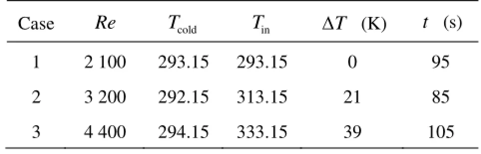
Table 1 Overview of the experiments

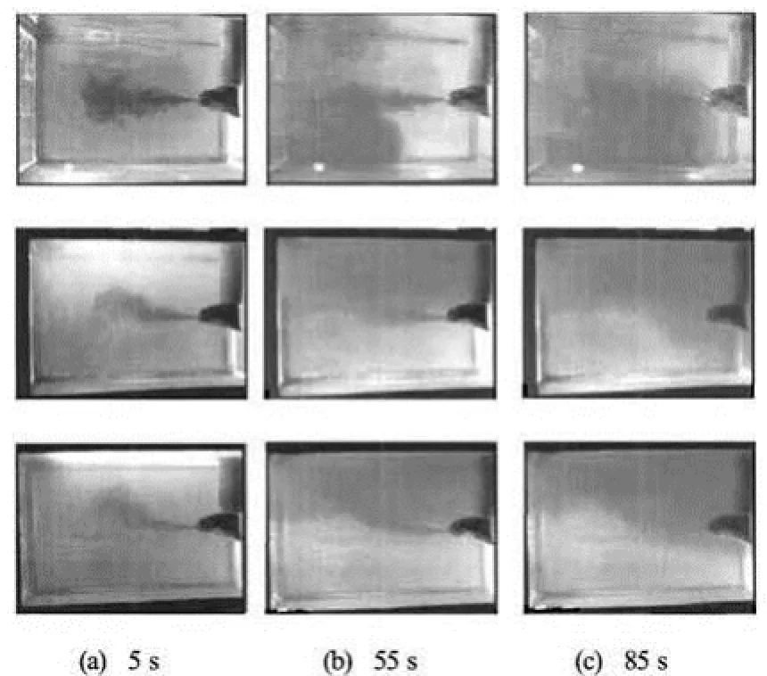
Fig.2 Visualization of flow structures for ΔT=0 K (1st row), ΔT=20 K (2nd row) and ΔT=40 K (3rd row)

The parameters used for the three cases of studies are listed in Table 1, where Re is the Reynolds num-ber,Tcoldthe temperature of the water in the tank at the beginning of the experiment,Tinthe temperature of the entering water, ΔT=Tin-Tcoldthe temperature difference between the hot water and the cold water andtthe total time of the visualization. For the three cases, the flow rate is 0.7 l/min and the inlet velocity is 0.3 m/s.

Visualizations are performed by using a digital video camera every five seconds. Figure 2 shows an example of visualization for the flow patterns during a draw-off test with an inlet flow rate of 0.7 l/min with three different inlet temperatures for the three cases. The buoyancy effects due to natural convection are clearly illustrated in Fig.2, such that for the isothermal case (ΔT=0 K), there is no buoyancy effect because there is no heat transfer, while for the second and third cases it can be observed that the red colored water (hot water) moves to the top of the tank depending on the temperature difference. Also, one can note that the buoyancy force of Case 3 ΔT=40 K is greater than that of Case 2 ΔT=20 K.

2. Mathematical formulations

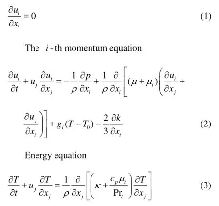
The problem of a 3-D vertical water jet entering water in a rectangular storage tank is considered. The RANS with the realizablekε- model are used for the modeling of the turbulent flow. The realizablekε- model included an eddy-viscosity formula and a model equation for dissipationεbased on the dynamic equation of the mean-square vorticity fluctuation. So, the governing equations of mass, momentum, energy and turbulence take the form:

Continuity equation

Turbulence kinetic energy ()kequation

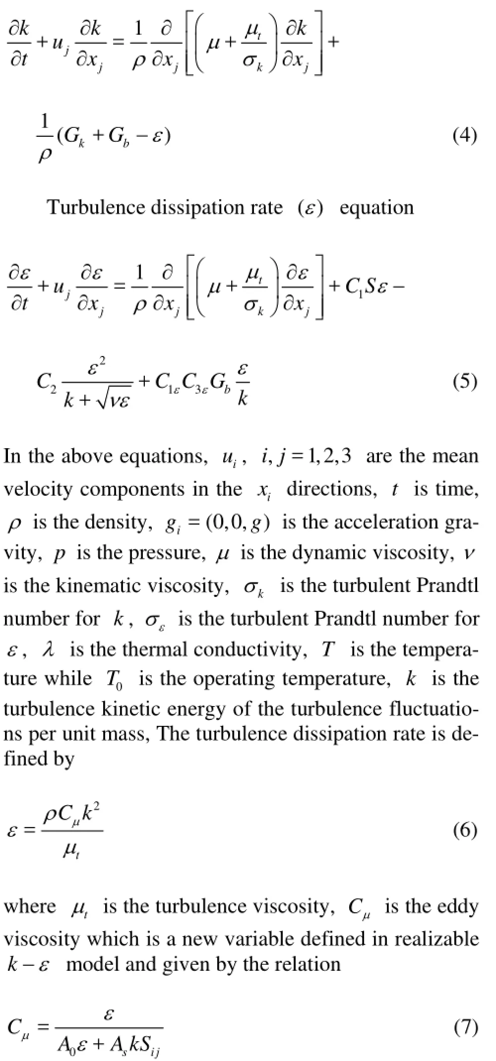
whereSis the modulus of the tensor of the mean strain rate which is defined by

is the generation of turbulence due to buoyancy.Prtis the turbulent Prandtl number for energy andβis the thermal expansion coefficient. The model constants of thek-εmodel are established to ensure that the model performs well for certain canonical flows.C1ε=1.44,C2=1.9,σk=1.0,Prt=0.85 andσε=1.2.

The turbulence intensity can be defined as the ratio of the magnitude of the root mean square (rms) turbulent fluctuations to the reference velocity

wherekis the turbulence kinetic energy andVis the reference velocity. The reference value specified should be the mean velocity magnitude for the flow. The velocity magnitude can be defined as the magnitude of the rms velocity components. Note that turbulence intensity can be defined in different ways. It is clear that the unit quantity ofVis velocity whileIis a dimensionless quantity, becausekhas a velocity square unit.

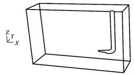
Fig.3 Model outline of the symmetrical half tank

3. Numerical investigations

The current problem is to visualize and to simulate the stratification of the hot water inside a water store. Symmetry is assumed in the vertical central plane of the tank, so for this model only half of the tank is modeled. Figure 3 shows the model outline for the symmetrical half tank with the dimensionsX×Y×Z=0.486 m×0.1375 m×0.29 m. Furthermore, the heat transfer through the walls of tank is not taken into consideration, i.e., the tank walls are adiabatic. These simplifications are considered to reduce the total number of grid elements in the numerical mesh. The meshes are built up of hexahedral map cells, and the number of grid elements used in the model is 50,975 cells for the “fine grid” or “grid-1” which was used in all calculations. Also, two other grid cases are used to compare the results with the fine grid, one of them is a coarse grid which has 15 310 cells while the other is fine also (named “grid-2”) and has 46 715 cells. Figures 4(a) and 4(b) illustrate the fine grid faces of theXZ- plane and theXY- plane, respectively. For the coarse grid, faces of theXZ- plane and theXY-plane are shown in Figs.5(a) and 5(b), respectively. The CFD code Fluent with the grid generation tool Gambit is used to model the flow in the tank by solving the momentum, turbulence and energy equations. The realizablek-εmodel was used for modeling of the turbulent flow and the buoyancy is modeled using the Boussinesq approximation.

Fig.4 Fine grid

Because the water inside the tank was at rest before starting the water injection, the initial values of all dependent variables are taken to be zero except the initial temperature which is taken to be 293.15oK.

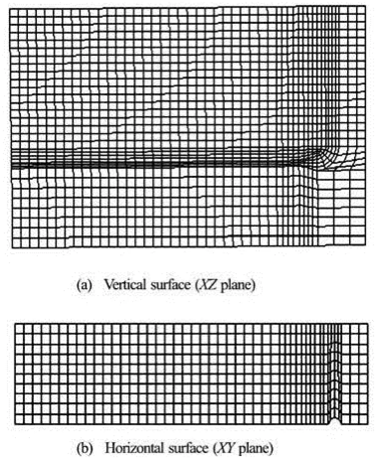
Fig.5 Coarse grid

Numerical solutions are obtained for unsteady flow while pressure, velocity, temperature and turbulence distributions inside the water tank are analyzed. In order to achieve convergence, the under-relaxation parameters are used on pressure, velocities, energy, turbulent viscosity, turbulence kinetic energy and turbulent dissipation rate.

Body force weighted discretization was used for pressure and the velocity-pressure coupling was treated using the PISO algorithm with the Skewness-Neighbor coupling correction parameters. A secondorder upwind scheme was used in the equations of momentum, energy, turbulence kinetic energy and turbulence dissipation rate. A 3-D segregated implicit solver with the implicit second-order scheme is used for unsteady formulations.

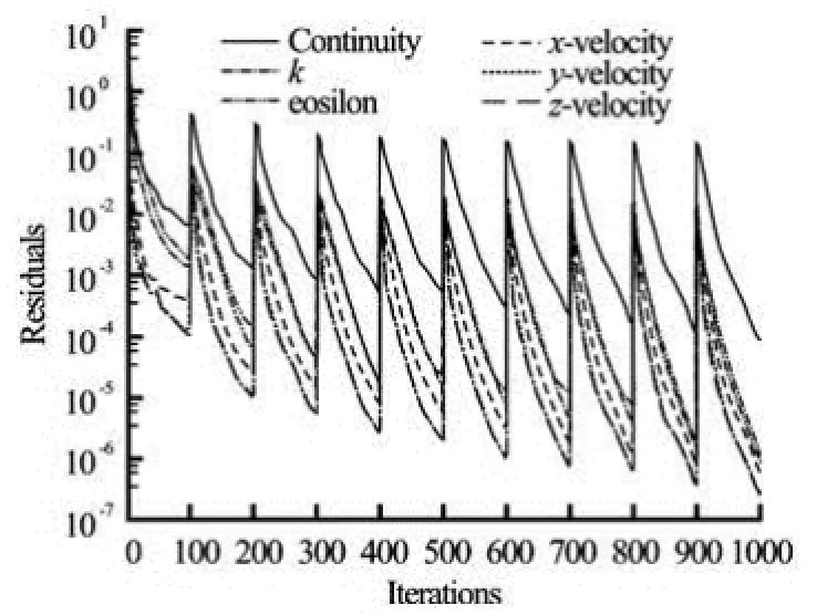
Fig.6 Residuals of the dependent variables for the first 1 000 iterations at =t1.0 s for Case 1

A time step of 0.1 s was used during the calculations. The heat losses from the tank have not been modeled. The number of iterations used in this problem is 100 iterations for each time step. That was enough to achieve the convergence for all physical quantities for the three different cases. Figure 6 shows the residuals of all dependent variables for the first 1 000 iterations (t=1s) for Case 1.

In this study, we will define two lines, and one of them is parallel to thex-axis with the dimensions (x=0-0.36,y=0.0001,z=0.1), this line lies in the core of the jet and will denoted byx. The other is parallel to thez-axis with the dimensions (x=0.1,y=0.0001,z=0-0.29) and is close to the wall opposite the jet entrance, which is also an important area.

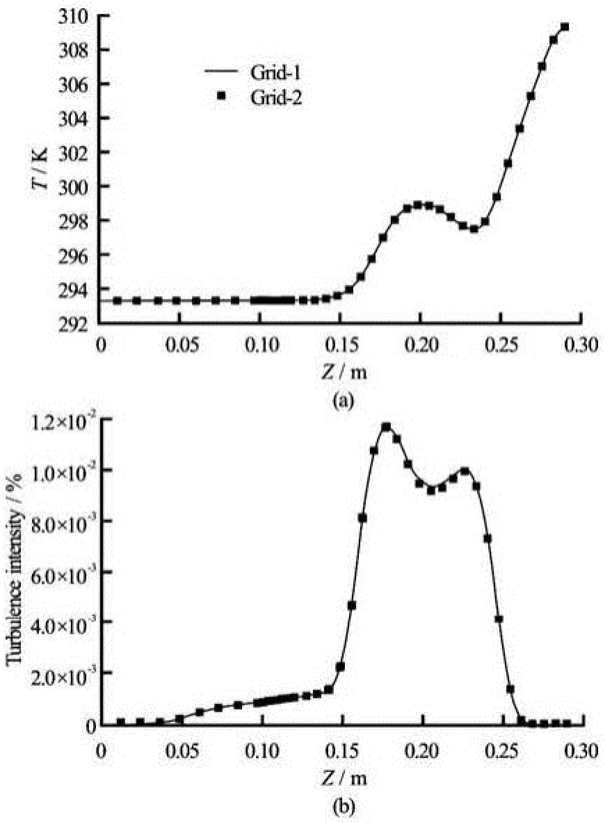
Fig.7 Temperature (a) and turbulence intensity (b) againstzwith different grid size at =t105 s, of Case 3

Figure 7 shows a comparison for the temperature and turbulence intensity, plotted as a function ofz, between the two different fine grid sizes “grid-1” and“grid-2” as defined above. These figures indicate that the solutions are not depending on the mesh for these cases. Also, Figs.8(a) and 8(b) illustrate a comparison between the fine grid size case and the coarse grid case for the static pressure and the temperature, respectively. From these figures it can be seen that the solutions for the two cases have the same behavior with only small quantitative differences.

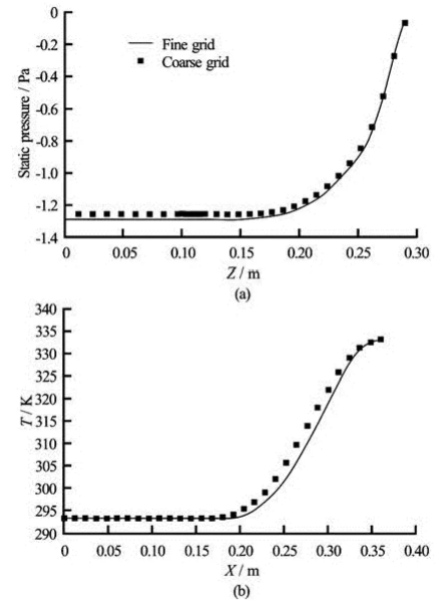
Fig.8 Static pressure (a) temperature profiles (b) as a function of x, with different grid size at =t75 s, of Case 3

Fig.9 Static pressure distribution as a function of x with various values of time for Case 1

4. Results and discussion

Static pressure along of the defined straight linexwith various values of the time for Case 1, ΔT=0 K, is shown in Fig.9. This figure indicates that the static pressure decreases as time increases alongx. Also, it can be seen that the static pressure in the jet area is greater than it in close to the wall.

The area between the inlet and the opposite wall has a small static pressure. It is interesting to note from Fig.9 that with advancing time steps the effect of time on pressure tends to vanish. This means that unsteady state tends to approach steady state.

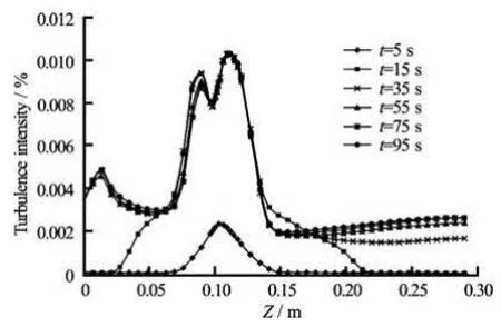
Fig.10 Turbulence intensity profiles as a function ofz, with various values of time for Case 1

Fig.11 Velocity magnitude profiles as a function ofzwith various values of time for Case 2

Figure 10 shows the turbulence intensity profiles as a function ofzwith various values of time for Case 1. It is observed that the highest turbulence intensity lies in the jet area. The top and the down parts of the tank have small turbulence intensity. Time effect on the turbulence intensity is non-uniformly depending on the turbulence state inside the tank. The distribution of the velocity magnitude as a function ofzwith various values of time for Case 2 is shown in Fig.11. It is noteworthy that the middle part (jet area) of the tank has the highest velocity magnitude while it is smaller in the top part and tends to vanish in the bottom part of the tank.

Fig.12 Temperature profiles as a function of z with various values of time for Case 2

Figure 12 shows the temperature distribution as a function ofzwith various values of time for Case 2. It is clear that the top part of the tank has the highest temperature and the opposite is true for the bottom part where the temperature seems to be the same as the initial temperature of the tank (293 K). From the same figure it can be seen that the temperature increases as time increases.

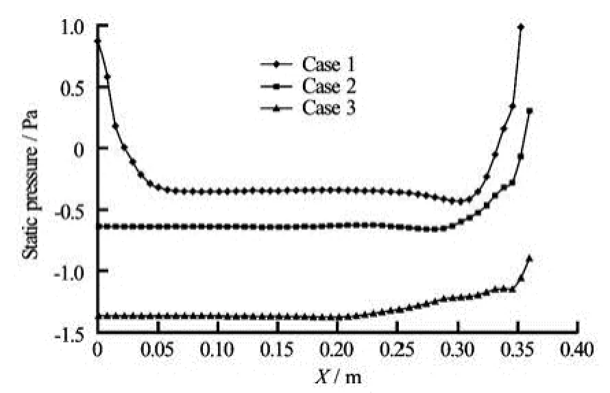
Fig.13 Static pressure profiles as a function of x with temperature differences =TΔ0 K,20 K,40 K at t=85 s

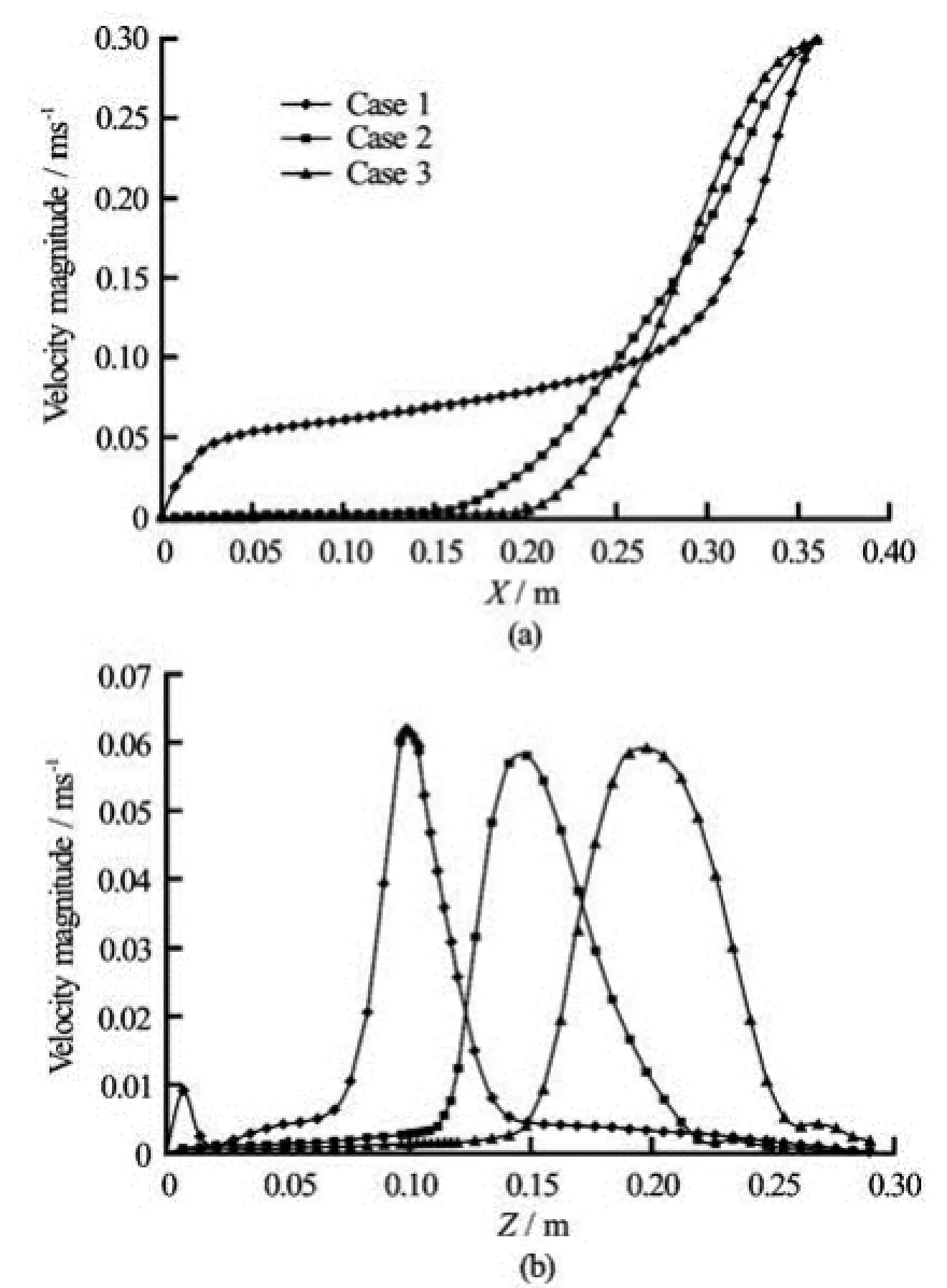
Fig.14 Velocity Magnitude profiles as a function of (a) x, (b) z with different temperature differences at t=85 s

A comparison between the static pressure profiles for the three cases of temperature differences, ΔT=0 K, 20 K, 40 K as a function ofxare shown in Fig.13 att=85 s. Figure 13 shows that the static pressure profiles along the linexdecrease as the temperature difference increases, and that the highest pressure for each case lies in the inlet area.

In Figs.14(a) and 14(b) the velocity magnitude profiles are plotted as a function ofxandz, respectively plotted for different temperature differences ΔT=0 K, 20 K, 40 K att=85 s. Figure 14(a) indicates that the velocity magnitude alongxclose to the wall for Case 1 is higher than for the second and third cases. This because the linexlies at the center of the jet for Case 1, while for the second and third cases the position of the jet area lies abovexaccording to buoyancy effect. From Fig.14(b), it is noteworthy that the position of the highest velocity magnitude depends on the position of the jet area that is shifted by buoyancy force in terms of temperature difference.

The temperature profiles as a function ofzare shown in Fig.15 for three temperature differences ΔT=0 K, 20 K, 40 K att=85 s. From Fig.15 it can be seen that the temperature is increased by raising the temperature difference especially in the top of the tank, while there is no difference at the tank bottom.

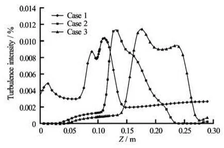
Fig.16 Turbulence intensity profiles as a function of z for different temperature differences at t=85 s

Figure 16 shows the turbulence intensity profiles as a function ofzfor different temperature differences ΔT=0 K, 20 K, 40 K att=85 s. From Fig.16 one can see that the position of the highest turbulence intensity depends on the temperature difference. The highest turbulence intensity lies in the jet area, thus forCase 1, ΔT=0 K, in the position around the inlet (because in this case there is no buoyancy force). The position of the highest turbulence intensity of Case 2 ΔT=20 K lies above the position of Case 1, and the position of the highest turbulence intensity of Case 3 ΔT=40 K lies above the position of Case 2.

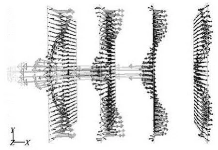
Fig.17 Velocity vectors in parallel vertical XY-plane x=0.1, x=0.2, x=0.3 and x=0.4 for Case 3, at 85 s

Figure 17 shows the velocity vectors on the parallel verticalXYplanesx=0.1,x=0.2,x=0.3 andx=0.4 for Case 3 at 85 s. It is obvious that, the jet area has the highest velocity. After impacting the opposite wall the water returns above and below the jet.

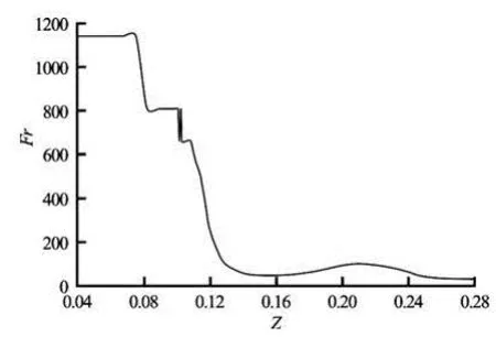
Fig.18 Internal Froude number as a function of z for Case 2

P hysical pro perties o f water such a s den sity, dynamicviscosity,thermalconductivityandspecific heat are expressed as functions of temperature using the interpolation method in the temperature range 293.15 K-313.15 K for Case 2:

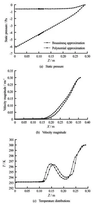
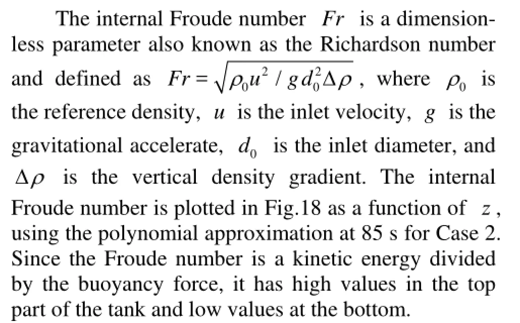
Fig.19 Comparison between Boussinesq and polynomial approximation at t=85 s for Case 2

The purpose of this section is to compare between this approximation and the Boussinesq approximation which is used above as shown in Fig.19. The results indicate that the distribution of velocity and temperature have the same behavior with small quantitative differences for the two approximations, while the behavior of pressure distribution as a function ofzis different (see Fig.19(a)). This is because in the Boussinesq approximation density varies only in the buoyancy force term in momentum equation and is considered constant in the other terms, while in the polynomial approximation the density varies always as a function of the temperature. Since the pressure term is divided by density, it should be affected by variation of density, which leads to a more realistic pressure distribution.

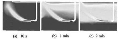
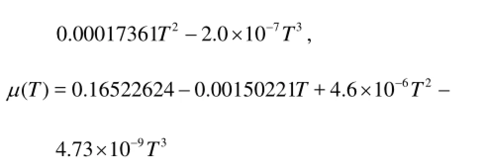
Fig.20 Contours of the temperature, for times 10 s, 1 min and 2 min, for Case 3

A good prediction of the stratification phenomena is shown in Fig.20. Contours of the temperature, at times 10 s, 1 min, 2 min of injection for Case 3 are plotted. It is observed from this figure that the layers of temperature appear early after a few seconds and become more clearly after a while. Moreover, this figure indicates that the realizablekε- model can model this problem very well.

Figure 21 shows pictures of the experimental visualization, and the contours of the velocity magnitude through a vertical section (the symmetry plane), the vertical section =x0.1, the horizontal sections (=z0.06, =z0.1 and =z0.16 for Case 1, =z0.1, =z0.16 and =z0.27 for Case 3), at 65 s for Case 1 and at 75 s for Case 3. These figures provide a complete understanding of jet flow under the current conditions. It is noteworthy that the non-buoyant jet is a pure jet, or in other words it is momentum-dominated jet. However, the buoyancy effect takes place when we have a temperature difference and the jet takes a plume (or forced plume) shape in which both momentum and buoyancy have effect.

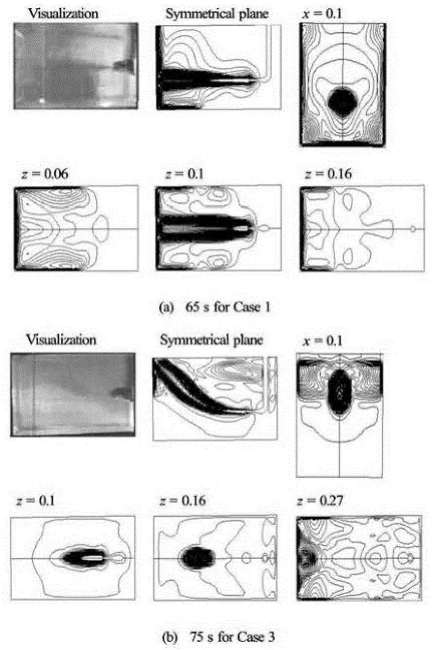
Fig.21 Experimental visualization, and contours of the velocity magnitude through vertical and horizontal sections

5. Conclusions

CFD treatments and experimental visualizations for the problem of a hot water jet entering horizontally into a water store containing cold water have been performed to illustrate the varying behavior of the thermal conditions in a solar store. Three temperature differences with the corresponding Reynolds numbers are considered. From this work one can conclude that:

(1) When these problems are treated as unsteadystate problems, after certain time the unsteady-state develops into the steady state.

(2) Jet entering the tank at the same temperature results in a regular spread of the jet inside the tank, while entering of a hot jet into the tank make the spread of the jet inside the tank depend on buoyancy forces due to the temperature difference.

(3) Thekε- turbulence model is suitable to decribe turbulent flow for this kind of problems, the Boussinesq approximation was used to model the buoyancy effect.

(4) Thermal stratification is verified through the temperature distribution.

(5) A polynomial approximation for the waterproperties as functions of temperature was compared to the results with the Boussinesq approximation.

[1] KNUDSEN S., FURBO S. and SHAH L. J. Design of the inlet to the mantle in a vertical mantle storage tank[C]. Proceedings ISES 2001 Solar World Congress. Adelaide, Australia, 2001.

[2] SHAH L. J., FURBO S. Entrance effects in solar storage tanks[J]. Solar Energy, 2003, 75(4): 337-348.

[3] JORDAN U., FURBO S. Investigations of the flow into a storage tank by means of advanced experimental and theoretical methods[C]. ISES Solar World Congress. Goteborg, Sweden, 2003.

[4] KNUDSEN S., MORRISON G. L. and BEHNIA M. et al. Analysis of the flow structure and heat transfer in a vertical mantle heat exchanger[C]. ISES Solar World Congress. Goteborg, Sweden, 2003.

[5] El-AMIN M. F., HEIDEMANN W. and MÜLLERSTEINHAGEN H. Turbulent jet flow into a water store[C]. Proceedings Heat Transfer in Components and Systems for Sustainable Energy Technologies. Grenoble, France, 2005, 345-350.

[6] El-AMIN M. F., SUN S. and HEIDEMANN W. et al. Analysis of a turbulent buoyant confined jet modeled using realizable model[J]. Heat Mass Transfer, 2010, 46(8): 943-960.

[7] PANTHALOOKARAN V., El-AMIN M. F. and HEIDEMANN W. et al. Calibrated models for simulation of stratified hot water heat stores[J]. International Journal of Energy Research, 2008, 32(7): 661-676.

[8] FUKUSHIMA C., AANEN L. and WESTERWEEL J. Investigation of the mixing process in an axisymmetric turbulent jet using PIV and LIF[C]. Proceedings 10th International Symposium Applications of Laser Techniques Fluid Mechanics, Lisbon, Portugal, 2000.

[9] AGRAWAL A., PRASAD A. K. Integral solution for the mean flow profiles of turbulent jets, plumes, and wakes[J]. Journal of Fluids Engineering, 2003, 125(5): 813-822.

[10] ARAKERI J. H., DAS D. and SRINIVASAN J. Bifurcation in a buoyant horizontal laminar jet[J]. Journal of Fluid Mechanics, 2000, 412: 61-73.

[11] O’HERN T. J., WECKMAN E. J.and GERHART A. L. et al. Experimental study of a turbulent buoyant helium plume[J]. Journal of Fluid Mechanics, 2005, 544: 143-171.

[12] El-AMIN M. F., KANAYAMA H. Integral solutions for selected turbulent quantities of small-scale hydrogen leakage: A non-buoyant jet or momentum-dominated buoyant jet regime[J]. International Journal of Hydrogen Energy, 2009, 34(3): 1607-1612.

[13] El-AMIN M. F., KANAYAMA H. Similarity consideration of the buoyant jet resulting from hydrogen leakage[J]. International Journal of Hydrogen Energy, 2009, 34(14): 5803-5809.

[14] El-AMIN M. F. Non-Boussinesq turbulent buoyant jet resulting from hydrogen leakage in air[J]. Internatinal Journal of Hydrogen Energy, 2009, 34(3): 7873-7882

[15] JIRKA G. H. Integral model for turbulent buoyant jets in unbounded stratified flows, Part 1: Single round jet[J]. Environmental Fluid Mechanics, 2004, 4(1): 1-56.

[16] JIRKA G. H. Integral model for turbulent buoyant jets in unbounded stratified flows, Part 2: Plane jet dynamics resulting from multiport diffuser jets[J]. Environmentai Fluid Mechanics, 2006, 6(1): 43-100.

10.1016/S1001-6058(14)60012-3

* Biography: EL-AMIN M. F. (1971-), Male, Ph. D., Research Scientist