Geometric Covariance Modeling for Surface Variation of Compliant Parts Based on Hybrid Polynomial Approximation and Spectrum Analysis＊

Tan Changbai(谭昌柏)，Hou Dongxu(侯东旭)，Yuan Yuan(袁园)，2＊

1.College of Mechanical and Electrical Engineering，Nanjing University of Aeronautics and Astronautics，Nanjing，210016，P.R.China;2.College of Computer Science，Nanjing Institute of Industry Technology，Nanjing，210046，P.R.China

1 Introduction

Compliant thin-walled part is widely used in the structures of automobile and aircraft.Because of its large size，complex shape and weak stiffness，compliant part tends to deform in the phases of forming，storage，shipment and assembly，and the real shape of part will deviate from its nominal position more or less.Moreover，the part variation coupling with various tool variations will create a stream of variations which propagate in flexible assemblies［1］.Actually，shape closure and force closure are both involved in flexible assemblies.Shape variation of compliant parts will introduce misalignmentsbetween the mating parts.Therefore，the shape variation of parts maybe results in the serious problems on the ultimate assembly quality and function of product.The importance of understanding the dimensional variation in flexible assemblies has been widely recognized in the industries such as automobile and aircraft manufacturing，and some issues including characterizing the compliant part variation and formulating the dimensional relations of part variation，tool variation and the assembly variation have become a popular research topic.A systematic study regarding the dimensional variation analysis in automobile assemblies is conducted at the University of Michigan.In the early，Liu and Hu［2］proposed a cantilever beam model for the spot welding process and conducted assembly variation predict using the Monte-Carlo simulation.There are some disadvantages in the cantilever beam model.The geometric structure of part is oversimplified and a simple beam is incapable to represent a complex 3D structure.The Monte-Carlo simulation is also time-consuming.To overcome the above shortcomings，Liu and Hu［3］introduced a linear elastic model by combining the finite element method and statistical analysis.Compared with Monte-Carlo simulation，statistical finite element method(SFEM)is more practical due to its high efficiency.Chang，et al［4］proposed an approach to simulate the assembly process and find the variation introduced into the assembly based on the part stiffness matrix.Sellem，et al［5］combined the results of Liu and Chang to develop a linear method that uses influence coefficients to find the variation of the parts.Zhang，et al［6］studied the riveting process of aircraft thin-wall structure，and a theoretical variation model of rivet shank and tail regarding the elastic and plastic deformation was established and validated by ABAQUS FEM simulation.Cheng，et al［7］investigated the positioning error of aeronautical thin-wall structures with the automated riveter systems.In the method，the riveting process is divided into two stages according to the fixture changing，and positioning error is developed based on the mismatch error analysis.In short，a lot of researches are conducted on the dimensional variation analysis in compliant assemblies.Hereinto，the part variation characterization plays a key role.

Merkley［8］introduced the concepts of material covariance and geometric covariance for tolerance analysis of flexible assemblies.The material covariance concerns the elastic deformation correlation of compliant parts and can be referred as the stiffness matrix of compliant parts often obtained by finite element tools.The geometric covariance is related to the level and correlation of original part variation，and a random Bezier curve method is developed to represent the noideal part profile.A major shortcoming of this method lies in its ignorance of the error patterns specific to part structure，forming process and materials.Under the constraint of tolerance band，a general random Bezier curve is used to define the relation of points，and the covariance of control points is only related to the curve order and parameter of sample points instead of the coordinates of control points.Thus，the covariance matrix of data points only depends on their parameters，and has nothing to do with the specific shape of curve.In other word，the covariance model by the random Bezier method ignores the inherent process-related error characteristics of compliant part，and merely utilizes the Bezier curve to guarantee the geometric continuity of adjacent points.Later，Bihlmaier［9］introduced a tolerance analysis method for flexible assemblies using spectral analysis，in which the autocorrelation function is used in frequency spectrum analysis to model random surface variation，which is related to the specific variation pattern.Stewart［10］proposed a polynomial-based model of geometric covariance for surface variation.Tonks，et al［11，12］proposed a hybrid model in which Legendre polynomials and average auto spectrum were used to model the surface covariance with longer and shorter wavelengths respectively.Unfortunately，these approaches are far from perfection，and there still exist some deficiencies or disadvantages.For example，the frequency spectrum method works well in modeling the surface waviness with shorter wavelengths，but it is not applicable for model surface warping with wavelength longer than the length of part.The frequency spectrum method also supposes all the surface points share the same standard deviation，but it is inconsistent with the actual situation of variation.For the polynomial method，the order of polynomials must be less than the number of sample points.The polynomial method is also incapable of formulating geometric covariance of surface exhibiting sinusoidal variation.A possible solution to represent the geometric covariance of surface variation is combing various types of polynomials.In the supposed scenario，the geometric covariance of surface warping and waviness can be modeled by Legendre polynomials and sinusoidal polynomials respectively.Unfortunately，the relevant research results do not reveal the methodology of retrieving the weighting coefficients of each component in mixed polynomials.

In this paper，a comprehensive approach of geometrical covariance modeling for surface variation of compliant part will be developed.Based on Fourier polynomial theory，the approach combines Legendre polynomials and sinusoidal polynomials to approximate surface variation with diverse spectrum characteristics.In the approach，surface warping and surface waviness will be focused on and represented by a series of mixed polynomials.Spectrum analysis will wherein be used to acquire the frequency and the amplitude of surface variation.A geometric covariance model respects the continuity and statistical characteristics of surface variation will ultimately be established in a comprehensive way.

2 SFEM of Tolerance Analysis and Geometrical Covariance Modeling

2.1 SFEM of tolerance analysis in flexible assemblies

To study the elastic deformation of compliant parts subject to forces，the finite element method is widely used to analyze the dimensional variation in flexible assemblies［13］.Basically，a typical assembly process can be divided into four phases by finite element method:Parts positioning，fixtures clamping，fastening and fixtures release，as seen in Fig.1.According to the hypothesis of small linear elastic deformation，a linear relation can be deduced between the initial mating gaps δa，δband assembly variation δcbased on the relation of closing forces Fa，Fb，and spring-back reaction force Fc.The linear elastic solution for dimensional variation analysis for flexible assemblies is illustrated as follows

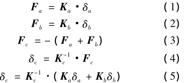
where Ka，Kband Kcare respectively the stiffness matrixes of Part a，Part b and Assembly c.The mating gaps δa，δband δcare the synthetic result of part variations，position variations and clamping variations，and these variants are regarded as the input variations of flexible assembly by the finite element method.This model focuses on the approach of characterizing the surface variations of parts.

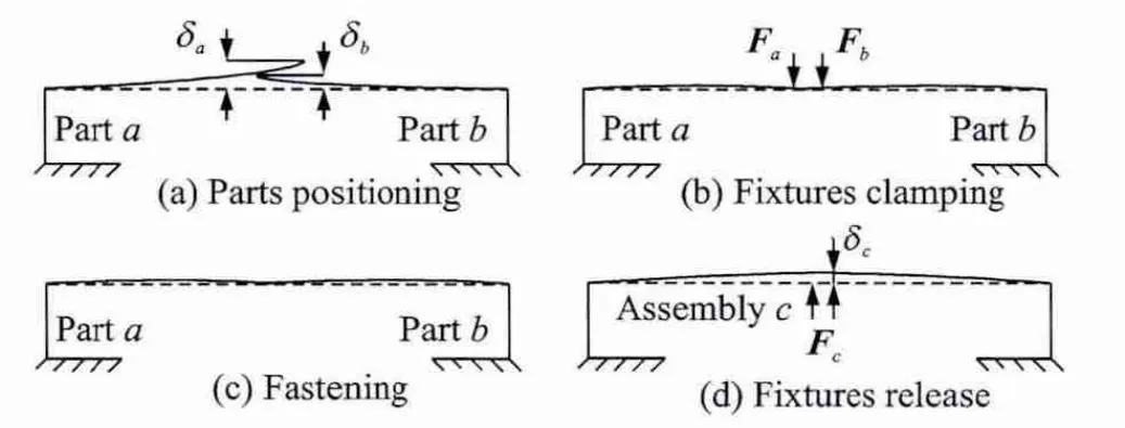
Fig.1 Decomposition of flexible assembly process

The linear model as Eq.(5)enables an insight into the dimensional variation in flexible assemblies from a statistical viewpoint.In the SFEM［14，15］，the mean and variance of dimensional variations to parts and assemblies are specially analyzed.The SFEM provides a high efficient linear algorithm to predict the mean and variance of assembly variation directly from the mean and variance of parts or tools variations.The mean is expressed as Eq.(6)

The variance is expressed as Eq.(7)

where μi(i=a，b，c)denotes the mean of part variations and assembly variation at the mating points，Σi(i=a，b，c)the geometric covariance of parts variations and assembly variation at the mating points.For a compliant part，under the constraint of geometric continuity，variations of points on surface within a tolerance zone are correlated to each other，and the correlation of variations within a part surface is closely related to the distribution of assembly variation.

2.2 Geometric covariance modeling by hybrid polynomials approximating

Certain polynomials maybe specialize in describing one class of shapes.Unfortunately，the surface variations of compliant parts usually involve complicated shape characteristics.A hybrid polynomials representation can be effective，in which various types of polynomials are adopted to approximate the surface variations with different multi-frequency domain characteristics.The produced polynomial model shares the same variances at sampling points，but establishes a specified correlation among these points.Generally，an orthogonal polynomial series will be chosen and used as the basis functions in a generalized Fourier series.The hybrid polynomial approximation provides a powerful tool to model the complicated surface variation.Firstly，considering a random and uncorrelated point set f(xi)，i=1，…，n，it can be transformed into a correlated point set f(xi)*，i=1，…，n，by applying a transformation matrix S.It is determined by the discrete Fourier decomposition of the actual profile on surface

The actual profile on surface builds the correlation of surface variation at sampling points.As illustrated in Fig. 2， PA{=1，…，n}，PB{=1，…，n}are two sampling point sets of a profile in which each point moves within a tolerance zone.The points in PBare uncorrelated，while the points in group PAare correlated due to the constraint of surface geometric continuity.Thecorrelation of the points can be defined by a covariance matrix.

Fig.2 Correlation of sampling points

Then，based on the statistical theory，an equation can be deduced regarding the covariance of the correlated points f(xi)*［12］

where ΣGis the geometric covariance matrix of real profile variation relative to the ideal profile，which reflects the geometric continuity and statistical characteristics of surface variation.Because the sampling points are independent variants，Eq.(9)can be rewritten as

where Λ is a diagonal matrix and its diagonal elements are equal to the value of variances of the sampling points.In practice，the variances can be acquired by the designated tolerance.

3 Methodology

3.1 Geometric covariance modeling by hybrid polynomial approximation and spectrum analysis

The overall methodology for geometric covariance modeling is illustrated in Fig.3.

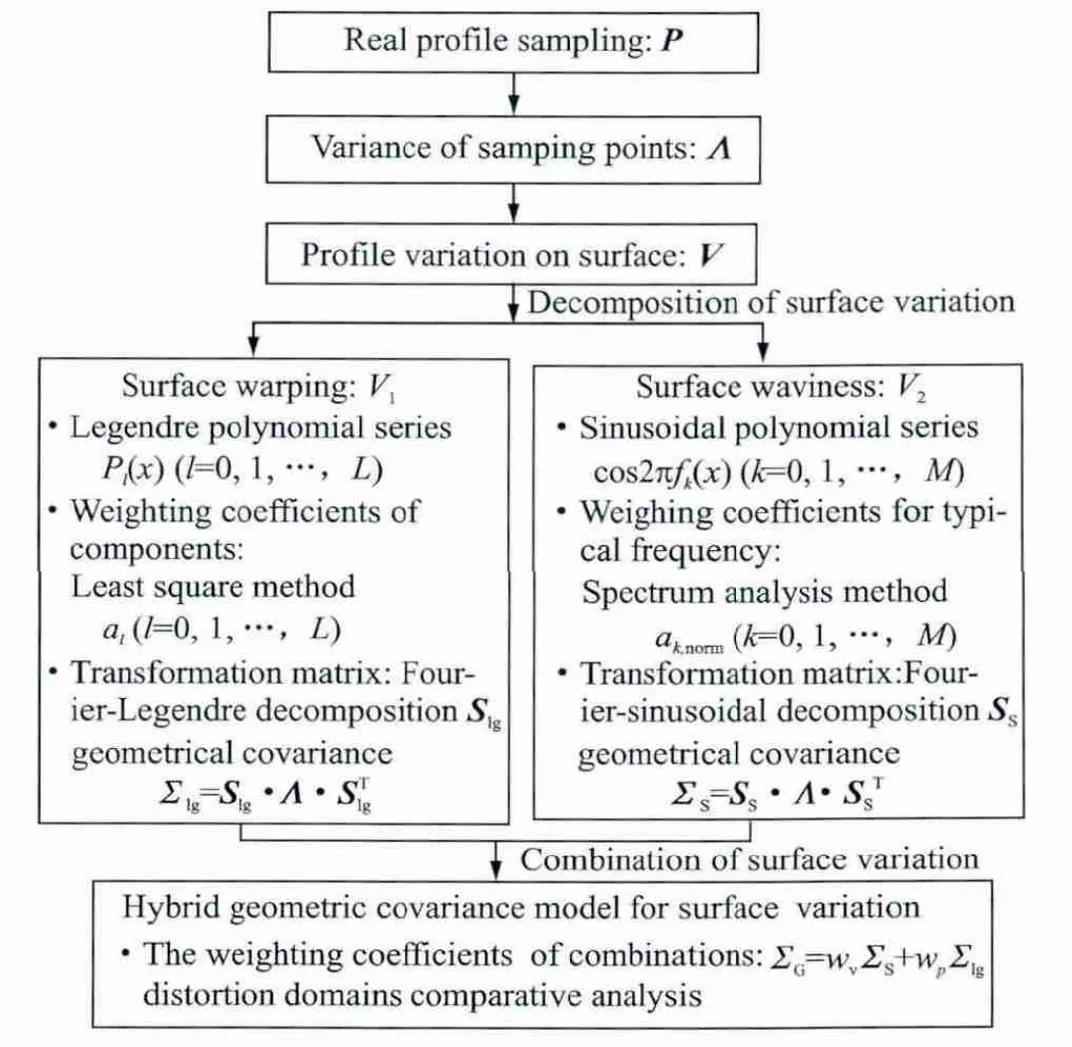
Fig.3 Methodology of geometric covariance modeling

Above all，the key profile on surface is selected to be sampled by discrete points(often by CMM or optical sensor).It should be noted that there are some regular patterns for the surface variation of compliant parts with similar structures or by a similar forming process.Therefore，the empirical data and model established by process experiments beforehand can be reliable and applicable for the future use.This fact is the foothold and significance of our research.It is critical to determine the diagonal matrix Λ and the transformation matrix S in the geometric covariance modeling.The diagonal elements of Λ can be statistically acquired if the experimental data are available，or be set by the tolerance band.In practice，a standard deviation is assumed to be one third the tolerance band.Coefficient matrix S is determined by the Fourier-Lengendre and Fourier-sinusoidal decomposition of the profile variation.Subsequently，the profile containing surface variation information will be approximated by hybrid polynomials.

According to the ratio ρ of part length L and variation wavelength λ，the surface variation can be decomposed into three basic modes［16］:(i)Surface warping(ρ ≤ 1);(ii)Surfacewaviness(1＜ρ≤5);(iii)Surface roughness(ρ＞5).Surface warping and surface waviness are focused in this research because they play the major role in the formation of dimensional variation in flexible assemblies.Generally，the amplitude of surface roughness is much smaller，and its contribution to the ultimate assembly variation can be neglected.The types of polynomials are carefully selected according to their capacities in shape representation of profile variations.Legendre polynomials are good at depicting surface warping［11］，and the weighting coefficients of components in a Legendre polynomial series，al，will be acquired by least square method.Furthermore，geometric covariance model for warping deformation is established by the method of Legendre polynomial decomposition and approximation.Subsequently，sinusoidal polynomials are chosen to represent the surface waviness.The weighting coefficients of components with different frequencies in a sinusoidal polynomial series，ak，norm，will be obtained by spectrum analysis.As a result，the geometric covariance model for surface waviness is developed.Finally，a hybrid geometric covariance model of surface variation is developed by combing the results of surface warping and surface waviness.The weighting coefficients of warping and waviness，wpand wv，are determined by the comparative analysis of distortion domains.

3.2 Covariance modeling for warping by Legendre polynomials approximating

Surface warping(ρ≤ 1)will be identified firstly and formulated by a series of Legendre polynomials.The transformation matrix Slgis solved by the Fourier-Legendre decomposition［12］.

The correlation of the sampling points on surface profile can be expressed by a Fourier-Legendre series

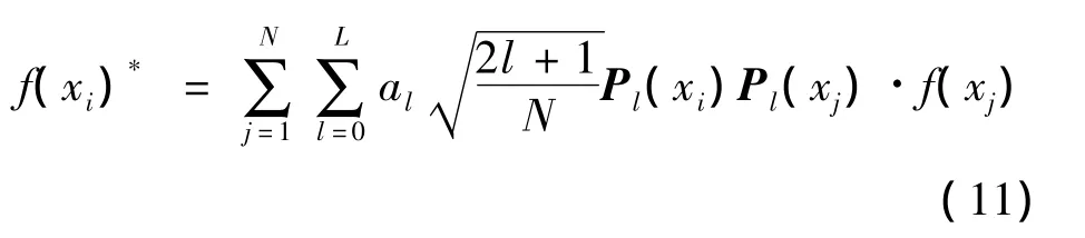
Therefore，the transformation matrix Slgis calculated by Eq.(12)

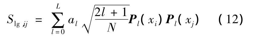
where N is the number of the sampling points，l the order of the Legendre polynomial，althe weighting coefficient of the l-order Legendre polynomial.This weighting coefficientcan be calculated by least squares approximation.In this research，a Legendre polynomial series with the increasing order to three is chosen，which exhibits excellent flexibility in modeling surface warping.

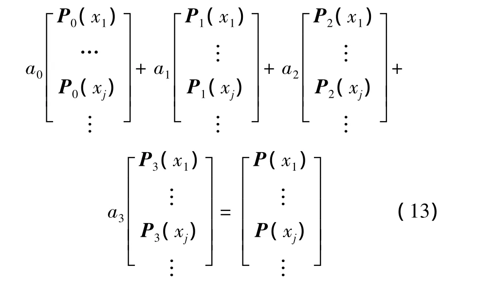
In Eq.(13)，Pl(xi)is the l-order Legendre polynomial，P(xi)the combination of Legendre polynomials of the first four orders.The profile data is fitted by Legendre polynomials of increasing order，subtracting each successive polynomial fit.The weighting coefficient of polynomial of each order is solved by least squares method，as follows

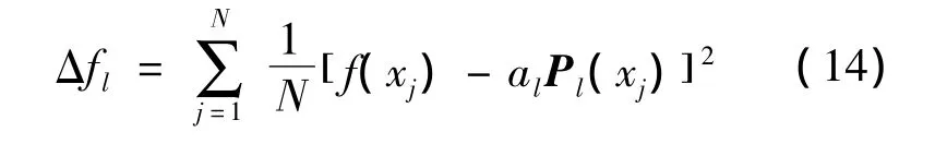
where f(xi)is the i-th sampling point on the real profile，Δflthe error function of least squares method.There exists a set of solutions for alto minimize the value Δfl.

The transformation matrix Slgcan be calculated by Eq.(12)，and the variance matrix Λ is also available.The geometric covariance for surface warping can be written as Eq.(15)

3.3 Covariance modeling for waviness by sinusoidal polynomials approximating and spectrum analysis

Surface waviness(1＜ρ≤5)will be approximated by sinusoidal polynomials of increasing order，and the transformation matrix SScan be acquired by the Fourier-sinusoidal decomposition［17］.

The correlation of the sampling points can be expressed by Fourier-sinusoidal series as Eq.(16)

The transformation matrix SSis calculated by Eq.(17)

In Eq.(17)，N is the number of sampling points，fkthe frequency of the sinusoidal polynomial，akthe weighting coefficient of the sinusoidal polynomial with the specified frequency.

The frequency information is difficult to acquire directly from the variation signal subtracting the Legendre polynomial fit.The method of solving the weighting coefficients in the Legendre polynomials approximating is not applicable here.Alternately，a spectrum analysis method is proposed according to the characteristics of surface waviness.

The discrete sampling points indicating surface variation can be viewed and treated as discrete digital signals.Fourier analysis［18］plays a very important role in discrete signal analysis，and provides a powerful tool to map the time domain analysis mode to frequency domain analysis mode.A variety of fast algorithms are available for discrete Fourier transform，which greatly improve the real-time and convenience properties of digital signal processing.This section will discuss the spectrum analysis of surface variation by fast Fourier transform(FFT)algorithm based on the Matlab toolbox［19］.

As shown in Fig.4，the spectrograms of a superposition signal from the sampling points.The signal is stacked by various sinusoidal signals with different frequencies.The frequency and amplitude information is revealed by the spectrogram，and the weighting coefficient of each basis function can be determined.In this case，the profile variation is stacked by four kinds of sinusoidal polynomials with different frequencies，f1，f2，f3and f4，and the weighting coefficients are depicted by Eq.(18)

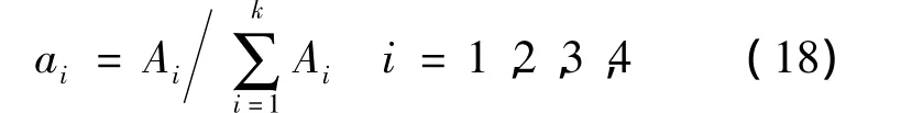
where Aiis the wave amplitude with the frequency fi.

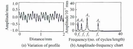
Fig.4 Spectrum analysis by FFT

In the spectrum analysis by FFT，there are two key points:(i)Frequency leakage;(ii)Frequency resolutions.By FFT，the original signal is truncated by window functions.For a component of particular frequency，without an integral wavelength in the sampling window，the method will produce a large distortion.In such case，the energy that should focus on a particular frequency is scattered to the nearby frequency domain and produced frequency leakage［20］.Therefore，there will be serious frequency leakage for surface warping whose wavelength is longer than the part length.That is why the spectrum analysis is not applicable when calculating the weighting coefficients of surface warping.Actually，the frequency leakage of warping can lead to a serious interference for the subsequent spectrum analysis of surface waviness.The component in waviness signal whose amplitude is small may be overwhelmed by leakage signal of warping.This problem is skillfully solved in this paper by separating the warping signal from the whole surface variation by the Legendre polynomial approximation.Thus，the spectrum analysis method is applicable to acquire the weighting coefficients of each component in surface waviness.The frequency resolution reflects the identification capacity between adjacent frequencies in FFT.When a key profile on surface is sampled at a sampling rate lower than two times of the maximum frequency in this profile，some frequency information must be lost in the spectrogram of spectrum analysis.Fig.5 illustrates two different results of spectrum analyses for the same profile at different sampling rates.The lower sampling rate can not distinguish the adjacent frequency.In our research，a method of high frequency sampling rate is adopted to improve the quality of spectrum analysis.

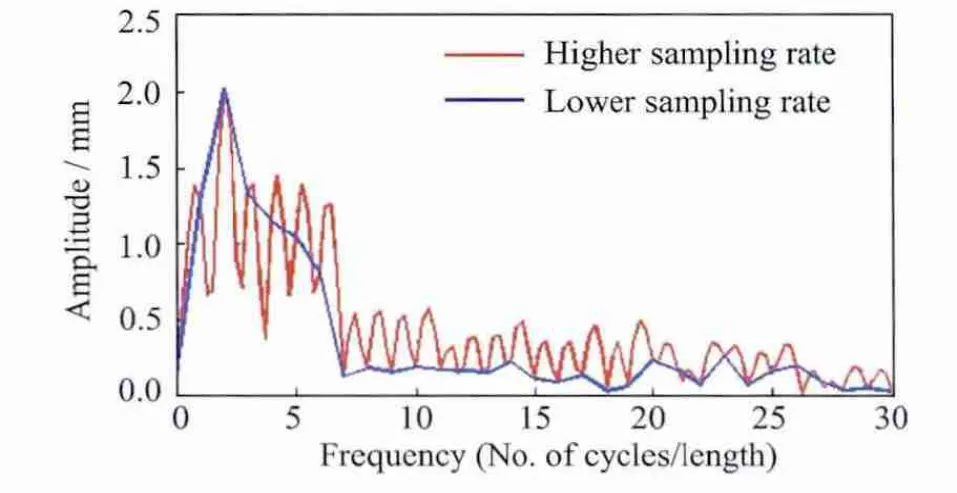
Fig.5 Spectrogram with different frequency resolutions

In this way，the weighting coefficients of each component in a sinusoidal polynomial series can be achieved by spectrum analysis.The geometric covariance matrix by the sinusoidal polynomial approximating is written as Eq.(19)

3.4 Hybrid geometric covariance model for surface variation

Surface variation in the flexible components can be classified as three types，warping，waviness and roughness.In this paper，only the effects of surface warping and surface waviness are concerned in the synthesis of surface deviation，because surface roughness has little to do with the macroscopic dimensional variation in flexible assemblies.A hybrid covariance model of surface variation is developed by combing the geometric models of surface warping and surface waviness linearly.The geometric covariance matrix of surface variation，ΣG，is expressed as Eq.(20)

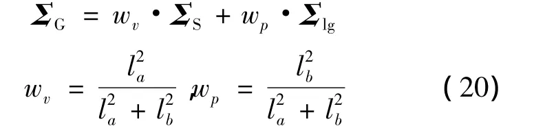
where a，b is respectively the variation band of waviness and warping.Since surface warping and waviness is already decomposed，the weights parameters laand lbcan be solved by the comparative analysis of distortion domain of the two components，as shown in Fig.6.

Fig.6 Comparative analysis of distortion domain

where yu1the upper limit of waviness，yl1the lower limit of waviness，yu2the upper limit of warping，yl2the lower limit of warping.

4 Verification

In this section，the proposed method is verified by a case study.As shown in Fig.7，the profile data at the assembly mating section are collected by CMM from a group of aluminum-alloy L-shape sheet metals.The thickness of these parts is 1 mm，and the profile length of the part is 150 mm，and 150 sampling points are equally selected for each part.

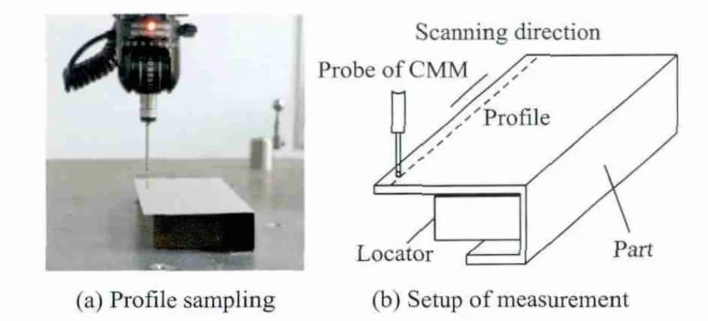
Fig.7 Profile measurement plan of sheet metals

The profile data are collected by CMM from six pieces of parts，shown in Fig.8(a).The profile data include both the random and non-random components.The non-random component involves the dimensional information of the nominal position and the mean errors.The random component reflects the profile errors deviating from the mean position.The geometric covariance of compliant sheet metals is modeled based on the random component，the random profile errors are shown in Fig.8(b).The geometric covariance model of surface variation is established by the proposed methodology.The curves of random profile errors are approximated by a hybrid Legendre and sinusoidal polynomial series，and the weighting coefficients of basis functions are determined based on the least squares method and the spectrum analysis.

As shown in Fig.9，the random profile errors are decomposed into warping and waviness.The error curves are firstly fitted by 0-order through 3-order Legendre polynomial consecutively，and the weighting coefficients of the basis functions are calculated by the least squares method，and the weighting coefficients and their mean values for theses profiles are shown in Table 1.The geometric covariance model for warping is established by Eqs.(12，15).

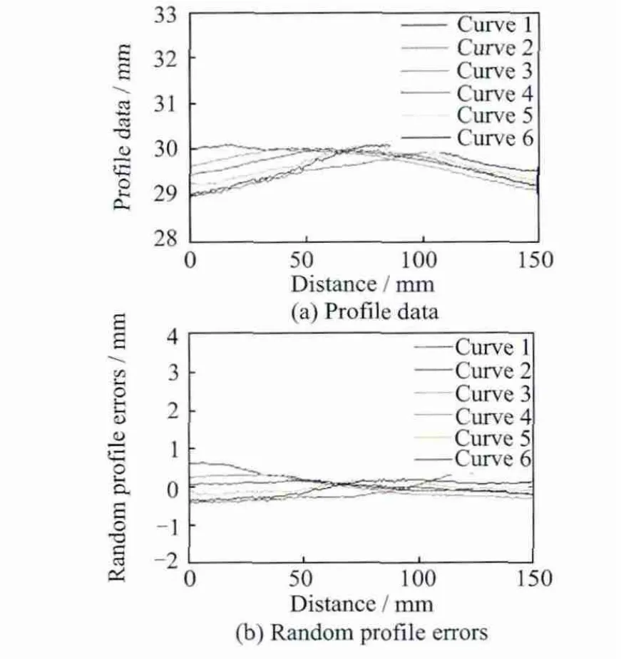
Fig.8 Surface variation collected by CMM

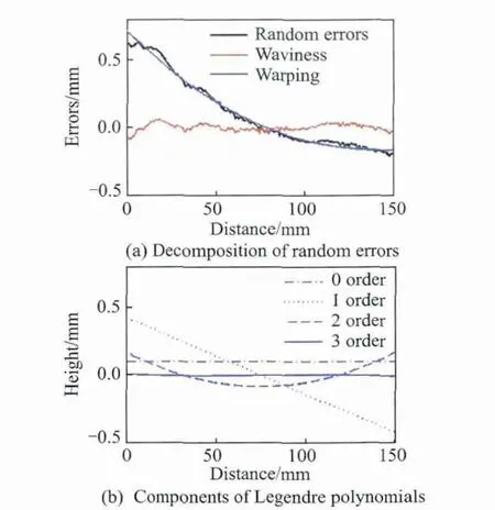
Fig.9 Legendre polynomials approximation of warping

Table 1 Weighting coefficients of Legendre polynomials

Subsequently，the residual errors of surface variation are approximated by a sinusoidal polynomial series.As shown in Fig.10，the spectrum analysis is conducted.The high-frequency components in the errors are viewed as surface roughness and filtered out directly.The after-filtered components are formulated by a sinusoidal polynomial series.The weighting coefficients can be acquired based on the amplitude-frequency curve in Fig.10.The weighting coefficients and frequencies of the six profiles are shown in Table 2.Therefore，the geometric covariance model for waviness is set up by Eqs.(17，19).

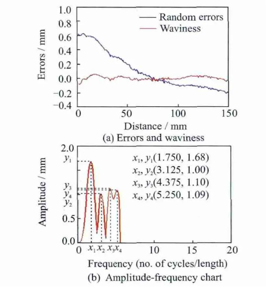
Fig.10 Spectrum analysis of surface waviness

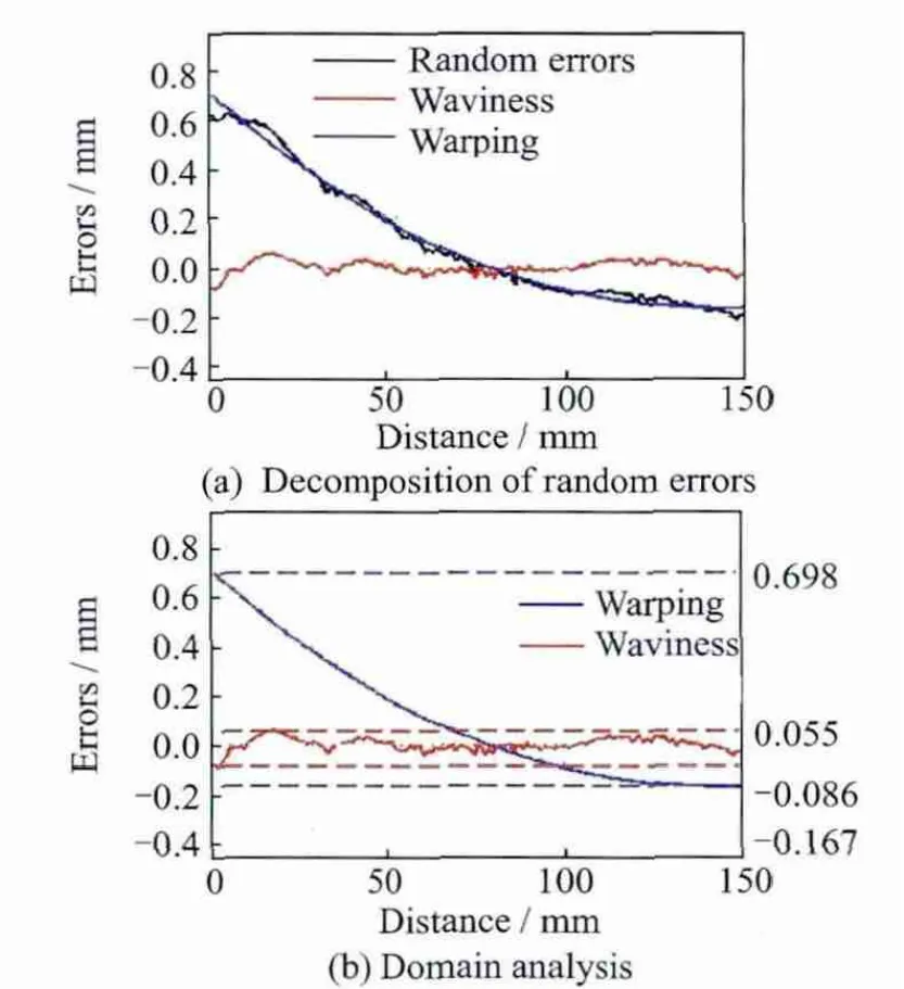
Fig.11 Comparative analysis of distortion domains

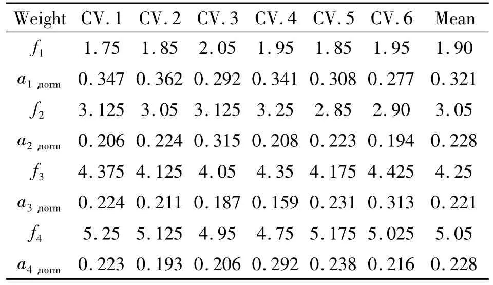
Table 2 Frequencies and weighting coefficients of sinusoidal polynomials

Subsequently，the results of the above polynomial approximating are combined，and a hybrid polynomial series is used to model the overall surface variation.By the comparative analysis of distortion domains，the variation bands of waviness and warping，laand lb，are listed in Table 3.Consequently，the comprehensive geometric covariance model for surface variation is developed by Eq.(20).

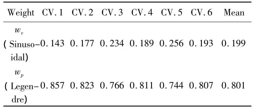
Table 3 Mixed weighting coefficients of surface warping and surface waviness

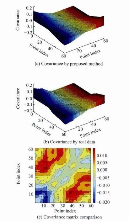
Fig.12 Comparative analysis of covariance matrix with statistical data

The variance matrices by the proposed method and the real data are illustrated as Fig.12.The height of histogram is proportional to the magnitude of covariance，which reflects the correlation level of the sampling points.Figs.12(a，b)denote the geometric covariance matrices by the proposed method and the sta-tistical data respectively.Fig.12(c)illustrates the plotted errors of covariance matrices between the two results.It reveals the proposed model can tightly fit the real statistical covariance of the real parts，with the maximum error 0.02(relative error 14%)and the average error 0.004(relative error 2.8%).It is also observed the geometric covariance model approximated the shape of statistical covariance matrix very well.

Furthermore，comparison analysis of covariance with two other methods is conducted to verify the advantages of the proposed method.Fig.13(a)denotes the covariance matrix formulated by the orthogonal polynomial method［12］and the plotted errors of covariance matrices between the orthogonal polynomial method and the real data.The maximum error is 0.02(relative error rate 14%)and the average error is 0.006(relative error rate 4.2%).Fig.13(b)denotes the covariance matrix solved by the hybrid method［11］and the plotted errors of covariance matrices between the hybrid method and the real data.The maximum error is 0.02(relative error rate 14%)and the average error is 0.007(relative error rate 4.9%).According to the comparison analysis，it can be concluded our method represents a better approximation to the real data，with a minimum average error.

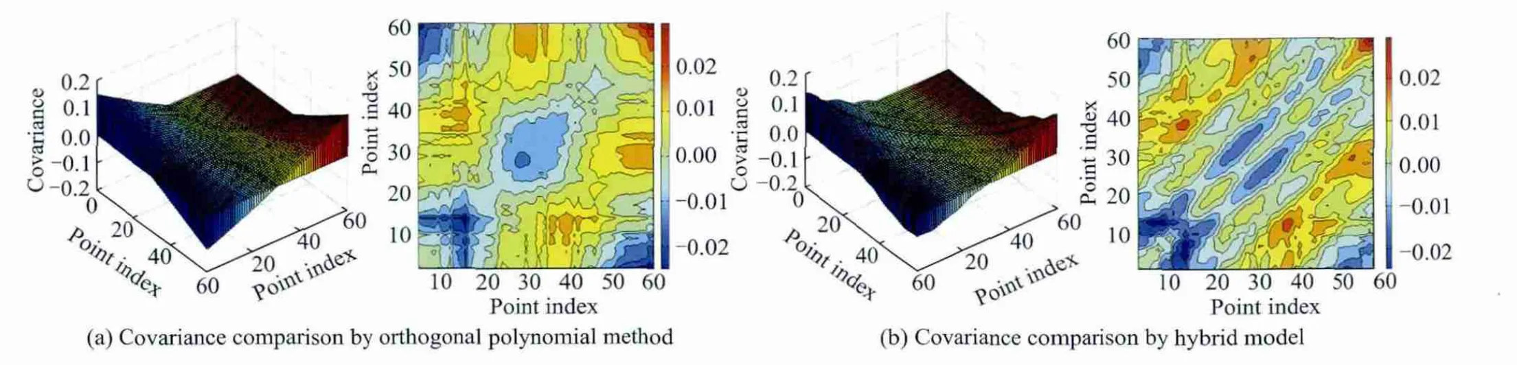
Fig.13 Comparative analysis of covariance matrix with other methods

5 Conclusions

For the statistical tolerance analysis in flexible assemblies，surface variation modeling for compliant parts is full of challenging.A flexible framework of geometric covariance modeling is proposed，in which warp and waviness are decomposed from the overall surface variation and dealt by the different schemes.A covariance model for surface warping is built based on the Legendre polynomial approximation.In a similar way，a covariance for surface waviness is established based on the sinusoidal polynomial approximation and spectrum analysis.Finally，a comprehensive geometric covariance representation of surface variation is developed by combing the two kinds of covariance models.The feasibility and advantages of this approach have been verified by a case study.

The presented framework is universal and extensible.In future work，a knowledge base including a variety of geometric covariance models for typical structures and manufacturing process should be established by specific process experiments，and can further be used in the dimensional quality prediction in new product development.

［1］ Hu S J.Stream of variation theory for automotive body assembly［J］.Annals of the CIPP，1997，46(1):1-6.

［2］ Liu S C，Hu S J.An offset finite element model and its applications in predicting sheet metal assembly variation［J］.Int J Machine Tools＆Manufacturing，1995，35(11):1545-1557.

［3］ Liu S C，Hu S J.Variation simulation for deformable sheet metal assemblies using finite element methods［J］.ASME Journal of Manufacturing Science and Engineering，1997，119(3):368-174.

［4］ Chang M，Gossard D C.Modeling the assemblies of compliant，no-ideal parts［J］.Computer Aided Design，1997，29(10):701-708.

［5］ Sellem E，Riviere A.Tolerance analysis of deformable assemblies［C］∥ Proceedings of the ASME Design Engineering Technical Conferences.Atlanta，USA:A-merican Society of Mechanical Engineers，1998:13-16.

［6］ Zhang Kaifu，Cheng Hui，Li Yuan.Riveting process modeling and simulating for deformation analysis of aircraft's thin-walled sheet-metal parts［J］.Chinese Journal of Aeronautics，2011，24(3):369-377.

［7］ Cheng Hui，Li Yuan，Zhang Kaifu.Efficient method of positioning error analysis for aeronautical thin-walled structures multi-state riveting［J］.Manuf Technol，2011，55(1/4):217-233.

［8］ Merkley K G.Tolerance analysis of compliant assemblies［D］.Provo:Dept of Mechanical Engineering，Brigham Young University，1998.

［9］ Bihlmaier B F.Tolerance analysis of compliant assemblies Using Finite Element and Spectral Analysis［D］.Provo:Dept of Mechanical Engineering，Brigham Young University，1999.

［10］Stewart M L.Variation simulation of fixtured assembly processes for compliant structures using piecewise-linear analysis［D］.Provo:Dept of Mechanical Engineering，Brigham Young University，2004.

［11］Tonks M R，Chase K W，Smith C C.Predicting deformation of compliant assemblies using covariant statistical tolerance analysis［J］.Models for Computer Aided Tolerancing in Design and Manufacturing，2007:321-330.

［12］Tonks M R，Chase K W.Covariance modeling method for use in compliant assembly tolerance analysis［C］∥ASME 2004 International Design Engineering Technical Conferences and Computers and Information in Engineering Conference.Salt Lake City:American Society of Mechanical Engineers，2004:49-55.

［13］Liu S C，Hu S J.Tolerance analysis for sheet metal assembly［J］.ASME Mech Des，1996，118(1):62-67.

［14］ Camelio J，Hu S J，Ceglarek D.Modeling variation propagation of multi-station assembly systems with compliant parts［J］.Journal of Mechanical Design，2003，125:673-681.

［15］Camelio J，Hu S J，Marin S P.Compliant assembly variation analysis using component geometric covariance［J］.Journal of Manufacturing Science and Engineering，2004，126:355-360.

［16］Soman S M.Functional surface characterization for tolerance analysis of flexible assemblies［D］.Provo:Dept of Mechanical Engineering，Brigham Young University，1999.

［17］Mortensen A J.An integrated methodology for statistical tolerance analysis of flexible assemblies［D］.Provo:Dept of Mechanical Engineering，Brigham Young University，2002.

［18］Qian T.Digital signal processing［M］.Beijing:China Machine Press，2004:65-76.(in Chinese)

［19］ Zhang X.The foundation and application of Matlab［M］.Beijing:China Electric Power Press，2009:41-45.(in Chinese)

［20］Jia M，Zhang H，Zhou J.Measuring and testing techniques［M］.Beijing:Higher Education Press，2001:58-68.(in Chinese)