Exact Polynomial Solutions of Schr¨odinger Equation with Various Hyperbolic Potentials∗

WEN Fa-Kai(温发楷),YANG Zhan-Ying(杨战营),,† LIU Chong(刘冲),YANG Wen-Li(杨文力), and ZHANG Yao-Zhong(张耀中)

1Department of Physics,Northwest University,Xi’an 710069,China

2Institute of Modern Physics,Northwest University,Xi’an 710069,China

3School of Mathematics and Physics,University of Queensland,Brisbane,QLD 4072,Australia

1 Introduction

It is well known that the exact solutions of the Schr¨odinger equation with diあerent potentials play an important role in mathematics and physics.[1−6]For example,Zhang studied exact polynomial solutions of second order diあerential equations and their applications;[1]Lee et al.applied some polynomial algebras to get exact solutions of general quantum nonlinear optical models;[2−3]Azad investigated the polynomial solutions of diあerential equations by the second order operators.[4]The exact solutions of the Schr¨odinger equation are very important in quantum mechanics since they contain all the necessary information of the quantum system,and some experimental alterable parameters,which can be used to check the numerical analysis of the equation.[7−8]Recently,the hyperbolic potentials have attracted great attention due to their wide range of applications in physics.[9−16]For instance,Oyewumi et al.investigated the bound-state solutions of the Rosen–Morse potential;[9]Wei et al.researched the Dirac equation with hyperbolic like potential;[11]Xie studied the energy spectra of a two-dimensional two-electron quantum dot with P¨oschl–Teller conf i ning potential;[13]Zhang et al.considered bound states of the Dirac equation with the Scarf-type potential.[15]

In general the stationary one-dimensional Schr¨odinger equation for a non-relativistic particle of mass m and energy E in a hyperbolic potential V(x)can be written as

follows:

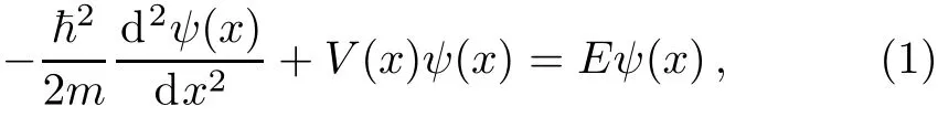
where

V0and d are the depth(or height)and width of V(x)respectively.If the parameters V0＞0,V(x)represents a potential well,see Fig.1;if the parameter V0＜0,V(x)depicts a potential barrier,see Fig.2.Downing presented the polynomial solutions of the case with V0＞0 and q=2 via reducing conf l uent Heun function to Heun polynomials.[6]In this work,we aim to present the general symmetric and antisymmetric polynomial solutions of all cases and discuss their applications in physics.

This paper is organized as follows.In Sec.2,we transform the Schr¨odinger equation into the conf l uent Heun equation by suitable transformations.Then,the general symmetric and antisymmetric polynomial solutions can be obtained via an eあective technique and the Functional Bethe ansatz method.We f i nd that all expressions for energy eigenvalues,wavefunctions and constraints can be unif i ed in one form for symmetric and antisymmetric solutions,respectively.Moreover,in order to ensure the energy to be real,we need to choose q=0,2 when V0＞0,and q=1,3 when V0＜0.In Sec.3,we present the wavefunction of the f i rst state,and discuss the wavefunctions of bound state.Finally,we draw conclusions in Sec.4.

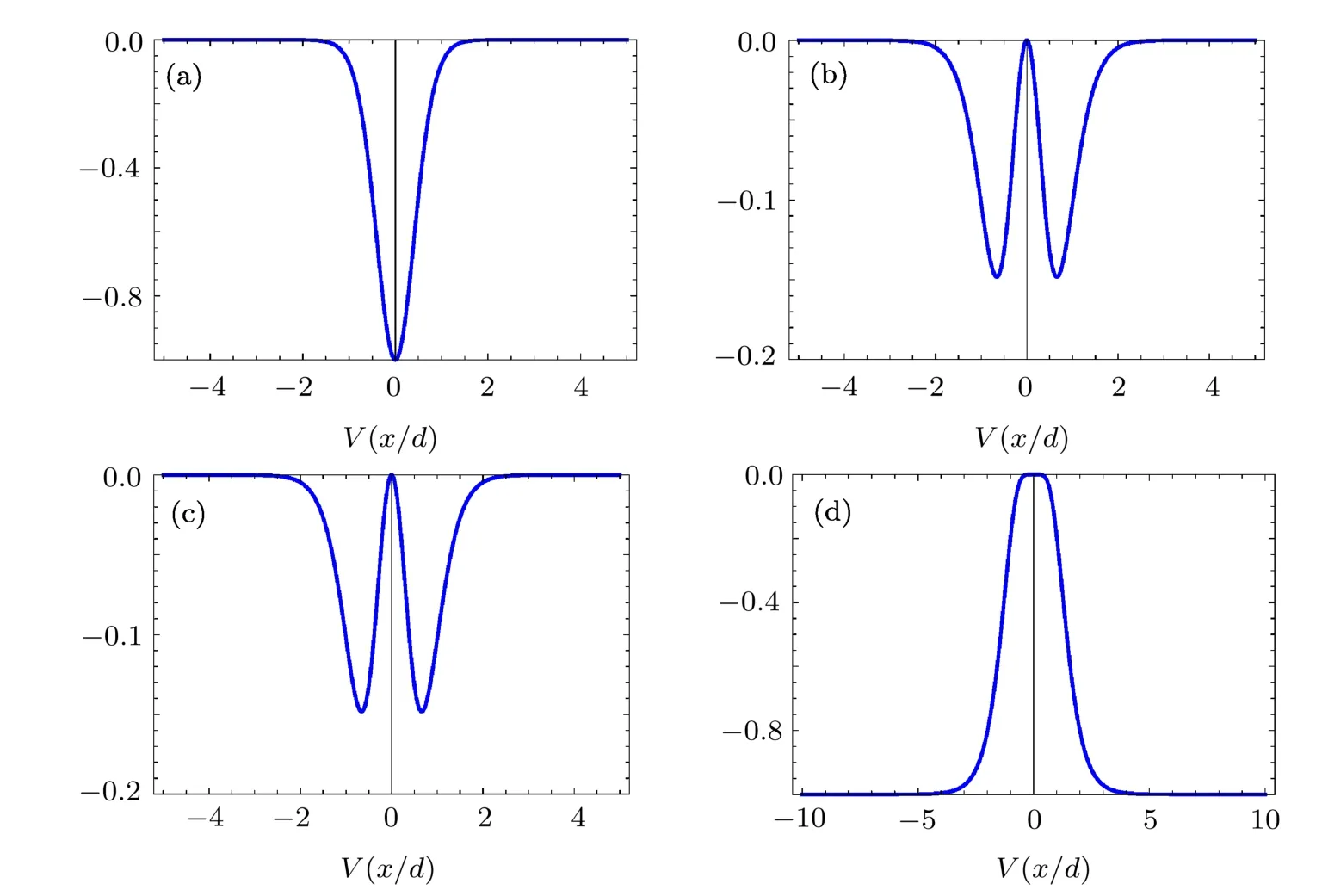
Fig.1 (Color online)The plot of the hyperbolic double-well potentials when V0＞0,(a)For q=0,(b)For q=1,(c)For q=2,(d)For q=3.

Fig.2 (Color online)The plot of the hyperbolic double-barrier potentials when V0＜0,(a)For q=0,(b)For q=1,(c)For q=2,(d)For q=3.

2 Reduction to a Conf l uent Heun Equation and General Exact Polynomial Solutions

Most of the theoretical physics known today is described by using a small number of diあerential equations,such as the hypergeometric equation,the Heun equation,etc.[17−21]In this section,we will transform the Schr¨odinger equation into conf l uent Heun equation by appropriate transformations.Heun equation is a secondorder linear diあerential with four regular singular points,which was initially studied by Heun.[17]It has several special cases of great importance in mathematical physics,namely the Lam´e,Mathieu,and Spheriodal diあerential equations.Recently,many researchers start focusing on Heun equation,for it has become increasingly widespread application in physics,such as quantum ring,black holes etc.

From Eq.(1),we have

where ε=2mE/ħ2,U0=2mV0/ħ2,z=x/d.

Upon making the change of variable η=1/cosh2(z),such that the domain−∞＜z＜∞maps to 0＜η＜1,we obtain

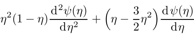
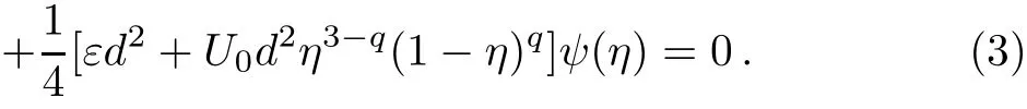
The last item contains the third power of the η,which brings great diきculties to solve the equation.Therefore,we make the following transformation

where A is a parameter to be determined.

Then,we obtain

Using the identical equation

we obtain

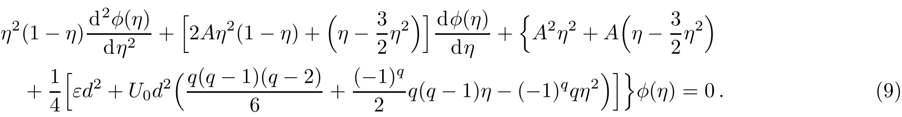
Choosing A to make the last item to be zero,i.e.

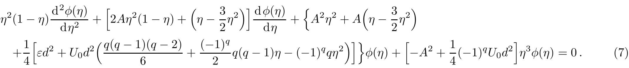
Therefore,Eq.(7)can be rewritten as follows

Applying the transformation

to transform Eq.(9)into the conf l uent Heun equation,where α is a parameter to be determined.

Then,we have

where

Choosing α to make the last item to be zero,i.e.

Finally,we get

Equation(13)is a conf l uent Heun’s diあerential equation,with regular singularities at η=0,1,∞.

Furthermore,in order to obtain symmetric and antisymmetric solutions in a unif i ed form,we make the following transformation

where β=0 or 1,and we obtain

Applying the procedure of Ref.[1],Eq.(15)has polynomial solutions of degree n=1,2,3,...

where the roots η1,η2,η3,...,ηnobey the Bethe ansatz equations

Moreover,the parameters α and A obey the following relation

Then,from Eqs.(12),(19),we obtain

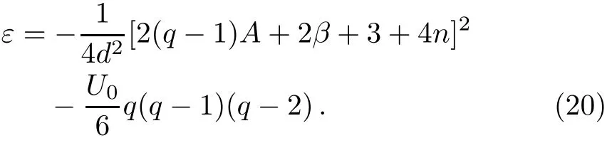
Therefore,the energy eigenvalues can be obtained as follows

Furthermore,we obtain the wavefunctions as follows

Thus,we have obtained the explicit expressions of energy eigenvalues,wavefunctions,and constraint conditions in unif i ed forms respectively.

For β=0,we obtain the energy eigenvalues and wavefunctions of symmetric state

For β=1,we have the energy eigenvalues and wavefunctions of antisymmetric state

Obviously,Eq.(24)indicates that the symmetric wavefunctions have even nodes and the most nodes is 2n for the n state.Similarly,Eq.(26)shows that the antisymmetric wavefunctions have odd nodes and the most nodes is 2n+1 for the n state.It is worth pointing out that symmetric and antisymmetric solutions were obtained by two initial variable transformations in Ref.[6],while we fi nd that the symmetric and antisymmetric solutions can be uni fi ed eあectively.Although our results are diあerent from Downing’s results when q=2,[6]we have veri fi ed that our polynomial solutions do indeed satisfy Eq.(1)as it is required.

3 Discussion on Wave Function withn=1 State

In Sec.2,we obtain the general polynomial solutions of wavefunction for the symmetric state and the antisymmetric state.In this section,for simplicity,we only consider the f i rst state(i.e.n=1),and higher states n=2,3,...can be obtained by the same recipe.

3.1 The First Symmetric State

The energy eigenvalue is

and the wavefunction is

There is a constraint between U0and d from Eqs.(17)and(18)as follows,

where

For simplicity,we fi x the width of potential d=1,and then obtain

Case 1 U0＞0,V(x)is potential well

Case 2 U0＜0,V(x)is potential barrier

Here we fi nd that the case with q=2,A=−α=−(A+7/2)/2 has symmetric wavefunctions of bound state.The energy is Es1= −(ħ2/8m)(−+7)2,and the wavefunction is

Figures 3(a)and 4(a)show that both wavefunctions are symmetric.As we increase the potential strengths,the wavefunctions become more tightly,namely the higher the potential strength the tighter the conf i nement,it is not hard to understand by the Heisenberg’s uncertainty relation.Moreover,we can see that a drop from two nodes to zero node in Figs.3(a)and 4(a),and the corresponding|Es1−V(x/d)min|become smaller see Figs.3(c)and 4(c).The change of the nodes is similar with some simple quantum systems such as one-dimensional inf i nite potential well,one-dimensional harmonic oscillator and so on.Furthermore,Fig.3(b)indicates that the probability density approximates to zero at the bottom of the potential well,while Fig.4(b)shows that the probability density is the largest at the lowest point of the potential well.This indicates that the particle tends to the bottom of the potential well with the potential strengths increase.

Fig.3 (Color online)The plot of symmetric state,with q=2,n=1,d=1,U0=149.574 25...,and energy Es1= −2.35309×10−10neV.(a)For wavefunction,(b)For probability density,(c)For hyperbolic double-well potential and energy level.

Fig.4 (Color online)The plot of symmetric state,with q=2,n=1,d=1,U0=595.838 65...,and energy Es1= −2.60744×10−9neV.(a)For wavefunction,(b)For probability density,(c)For hyperbolic double-well potential and energy level.

3.2 The First Anti-Symmetric State

The energy eigenvalue is

and the wavefunction is

There is a constraint between U0and d from Eqs.(17)and(18)as follows,

where

For simplicity,we let the width of potential d=1,and obtain

Case 1 U0＞0,V(x)is potential well

Case 2 U0＜0,V(x)is potential barrier

We obtain that the case with q=2,A= −/2,α=−(A+9/2)/2 has antisymmetric wavefunctions of bound state.The energy is Ea1= −(ħ2/8m)(−+9)2,and the wavefunction is

The results for the f i rst antisymmetric state have similar behavior with the f i rst symmetric state,as can be seen in Figs.5 and 6.We f i nd that the higher the potential strength the tighter the conf i nement,but note that a decrease in nodes from three to one.In physics,the f i rst antisymmetric state is similar with the f i rst symmetric state.

Fig.5(Color online)The plot of anti-symmetric state,with q=2,n=1,d=1,U0=426.232 048...,and energy Ea1= −1.16663×10−9neV.(a)For wavefunction,(b)For probability density,(c)For hyperbolic double-well potential and energy level.

Fig.6(Color online)The plot of antisymmetric state,with q=2,n=1,d=1,U0=1092.79897...,and energy Ea1= −4.97883×10−9neV.(a)For wavefunction,(b)For probability density,(c)For hyperbolic double-well potential and energy level.

4 Conclusion

We obtain the general polynomial solutions of the Schr¨odinger equation with various hyperbolic potentials,which can be reduced to the symmetric wavefunctions with β =0 and antisymmetric wavefunctions with β =1.Additionally,we must set q=0,2 with V0＞0 and q=1,3 with V0＜0 for the hyperbolic potential to ensure that the energy eigenvalue be real,which can be derived from the analytical expression of energy eigenvalue.Furthermore,we f i nd the number of wavefunction’s nodes decrease with the increase of potential strengths,and the particle tends to the bottom of the potential well correspondingly,for the bound states.

[1]Y.Z.Zhang,J.Phys.A:Math.Theor.45(2012)065206.

[2]Y.H.Lee,W.L.Yang,and Y.Z.Zhang,J.Phys.A:Math.Theor.43(2010)185204.

[3]Y.H.Lee,W.L.Yang,and Y.Z.Zhang,J.Phys.A:Math.Theor.43(2010)375211.

[4]H.Azad,A.Laradji,and M.T.Mustafa,Adv.Diあer.Equat.2011(2011)58.

[5]D.Agboola and Y.Z.Zhang,J.Math.Phys.53(2012)042101.

[6]C.A.Downing,On a Solution oftheSchr¨odinger Equation with a Hyperbolic Double-WellPotential,arXiv:1211.0913v1(2012).

[7]S.S.Dong,Mod.Phys.Lett.B 22(2008)483.

[8]S.Meyur and S.Debnath,Lat.Am.J.Phys.Educ.4(2010)587.

[9]K.J.Oyewumi and C.O.Akoshile,Eur.Phys.J.A 45(2010)311.

[10]X.Q.Zhao,C.S.Jia,and Q.B.Yang,Phys.Lett.A 337(2005)189.

[11]G.F.Wei,G.H.Sun,and S.H.Dong,Appl.Math.Comput.218(2012)11171.

[12]G.F.Wei and X.Y.Liu,Phys.Scr.78(2008)065009.

[13]W.F.Xie,Commun.Theor.Phys.46(2006)1101.

[14]M.Znojil,Phys.Lett.A 266(2000)254.

[15]X.C.Zhang,et al.,Phys.Lett.A 340(2005)59.

[16]G.F.Wei and S.H.Dong,Can.J.Phys.89(2011)1225.

[17]A.Ronveaux,Heun’s Diあerential Equations,Oxford University Press,New York(1995).

[18]M.Hortacsu,Heun Functions and Their Uses in Physics,arXiv:1101.0471v1(2011).

[19]P.P.Fiziev,J.Phys.A:Math.Theor.43(2010)035203.

[20]P.Loos and P.M.W.Gill,Phys.Rev.Lett.108(2012)083002.

[21]S.Hod,Phys.Rev.Lett.100(2008)121101.