Analytic solutions of the interstitial fluid flow models*
2013-06-01YAOWei姚伟LIYabei李亚贝
YAO Wei (姚伟), LI Ya-bei (李亚贝)
Shanghai Research Center of Acupuncture, Department of Mechanics and Engineering Science, Fudan University, Shanghai 200433, China, E-mail: weiyao@fudan.edu.cn
CHEN Nan (陈南)
School of Mathematical Sciences, Fudan University, Shanghai 200433, China
(Received September 6, 2012, Revised January 6, 2013)
Analytic solutions of the interstitial fluid flow models*
YAO Wei (姚伟), LI Ya-bei (李亚贝)
Shanghai Research Center of Acupuncture, Department of Mechanics and Engineering Science, Fudan University, Shanghai 200433, China, E-mail: weiyao@fudan.edu.cn
CHEN Nan (陈南)
School of Mathematical Sciences, Fudan University, Shanghai 200433, China
(Received September 6, 2012, Revised January 6, 2013)
In this paper, we present the analytic solutions of several continuum porous media models that describe the interstitial fluid flow in the interosseous membrane. We first compare the results of the Brinkman, Stokes and Darcy systems in describing the isotropic interstitial fluid flows. Our calculations show that the Stokes equations can well approximate the Brinkman equations when the Darcy numberDa≥0.2, while the Darcy model is an appropriate approximation to the Brinkman model in the interosseous membrane whenDa≤2× 10⁻⁴. Yet, in most cases, the anisotropy dominates the interstitial fluid. Therefore, we build an anisotropic Darcy model and show that an isotropic model can be used as a suitable approximation when the ratio between the transverse and longitudinal permeabilities is no larger than 20. Lastly, we take the blood flow in capillaries into consideration as well and introduce the coupled Stokes-Darcy system to describe the cases comprising both the capillary and the interstitial domain. Our results reveal that the profile of the interface exchange flow is not exactly in the linear form as was widely adopted in the numerical simulation, instead, the flux near the artery and the vein is more significant, which in turn results in the increase of the maximum horizontal velocity in the interstitial space while the outflow rate remains the same.
interstitial fluid flow, Brinkman system, Darcy system, Stokes system, coupled Stokes-Darcy system
Introduction
The interstitial fluid flow is the movement of fluid through the extracellular matrix of tissue, often between blood vessels and lymphatic capillaries, and is directly in contact with the cells. It provides a necessary mechanism for the transport of large proteins through the interstitium and constitutes an important component of the microcirculation[1]. Apart from its role in mass transport, the interstitial fluid flow also provides a specific mechanical environment for the interstitial cells, important to their physiological activities[2]. Manyin vitroexperimental and mathemaitcal models were set up to investigate the role of the interstitial fluid flow in guiding physiological activities[3-5]. The distribution of capillaries in a human body used to be assumed as a uniform network, and therefore the in vivo flow of the interstitial fluid was assumed to have no specificity. There were no direct in vivo measurements of the interstitial fluid flow except some observations[6,7]. For example, Li et al.[7]visualized the regional hypodermic migration channels of the interstitial fluid in human with the Magnetic Resonance Imaging (MRI). These channels were different from those of the lymphatic or blood vessels and were partially with the characteristics of the meridian. Numerical simulations in this field are few. The flow properties ofin vitroexperiments and numerical models were typically obtained based on experiential evaluations. Our previous studies on the anatomical structure of acupoints show that the tip of the acupuncture needle is normally placed near an interosseous membrane, and the capillaries in the interosseous membrane form a parallel array[8].
The interstitial fluid flow is a low-Reynolds-number flow in soft tissues composed of a porous matrix of fibrous materials and the proteoglycan. Most mathematical models deal with a regular parallel array of collagen fibrils as a continuum and are based on the Stokes, Brinkman and Darcy equations. Lee and Fung[6]showed that the Stokes equation could be satisfied everywhere except in a thin boundary-layer region near the fibrils surface. Based on the Brinkman equation, Tarbell used the softwares Fidap and Fluent in numerical simulations of the interstitial flow in vascular walls[9]. It is shown that the interstitial flow can be considered as a kind of communication signals between vessels and lower vascular smooth muscle cells. The Darcy’s law is wildly used to describe the porous media[6,10]. And a large number of numerical simulations for the interstitial fluid flows in interosseous membrane[11,12], based on such models show that the interstitial fluid flow plays an important part in the signals transmission and the structural reconstruction of osseous tissues. In the Brinkman and Darcy equations, the properties of the fibrous matrix are represented by a hydraulic permeabilitykp, that averages the flow resistance offered by the porous media across the entire flow domain. Many factors affect the tissue permeability; therefore, it is difficult to determine its accurate value which has to be evaluated in most cases. Yet, through numerical simulations, the estimated values in different cases are obtained, ranging from 10-10m2to 10-17m2[5,6].
In this paper, we deal with two issues. First, by adopting the Starling formula to describe the exchange of the fluid from the capillary, which serves as the boundary of the interstitial space, the analytic solutions of the Brinkman, Stokes and Darcy models in the single interstitial domain are obtained and the properties of the results of each model are analyzed. With the Brinkman model as the full description of the interstitial fluid flow, criteria are established of adopting the other two models as an appropriate approximation. An analytic solution for the anisotropic Darcy model is derived, and is compared with that of the isotropic model to determine when the latter can be used as an approximation for the anisotropic model. As the second issue, taking the influence of the blood flow in the capillary into consideration, we use the Stokes and Darcy equations as the governing equations to describe the blood and interstitial flows, respectively. We concentrate on the exchange flows at the interface, comparing it with the traditional hypothesis in the Starling formula. Furthermore, we analyze the interstitial flows, influenced by adding the blood flows in the capillary.
This paper is organized as follows. In Section 1, we present the three mathematical models to describe the flows in the interosseous membrane and the coupled Stokes-Darcy model to investigate the interaction between the blood flow in the capillary and the interstitial fluid flow, and derive the analytic solutions by the Fourier expansion. Section 2 is devoted to the analytic analysis and the numerical simulations based on these models. A summary of the present study is in Section 3.
1. Mathematical models and methods
1.1Brinkman, Stokes and Darcy systems for the interstitial flow
We start with a full description of the three models. The two-dimensional interstitial fluid domain [0,L]×[-H,H] is occupied by a porous media, the top and the bottom of which are the capillaries, as shown in Fig.1. We denote bykpthe permeability in the interstitial space,u=(u,v) the velocities,pthe pressure,μthe viscosity,ρthe density, 2Hthe distance between two neighboring capillaries andLthe length of capillary.

Fig.1 Conceptual domain for the interstitial space
To solve the mathematical models, we need to determine the boundary conditions. Since the fluid flows with a uniform velocity before entering and after leaving the domain which contains the capillaries, we thus assume that the derivatives of the horizontal velocities at the inlet and outlet are equal to zero, namely,

Unfortunately, with the Neumann boundary condition, the velocity is determined with an arbitrary constant, and the problem remains ill-posed. To overcome this flaw, we subtract a background flow to fix the horizontal velocity at the inlet as zero. On the other hand, at the top and the bottom of the interstitial space, we adopt the well-accepted Starling formula[13]

where
kc
is the permeability coefficient of the capillary walls,
σ
is the reflection coefficient of the protein, and
pc
,
pi
,
cζ
and
iζ
are the hydrostatic and osmotic pressures in the plasma and the interstitial fluid, respectively. Because of Eq.(2), the outlet velocity is no longer zero. Here, according to the Poiseuille’s Law
[13]
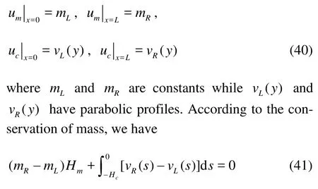
,
pc
will decrease linearly from the artery to the vein. Finally, to close the system, we impose the free-slip condition along the capillary walls, which is only required for the Stokes and Brinkman systems.
Here, the boundary conditions are as follows.
At the top and the bottom, the normal velocities are given,

Next, we are going to solve the three models to describe the interstitial flow. First, we introduce the non-dimensional variables
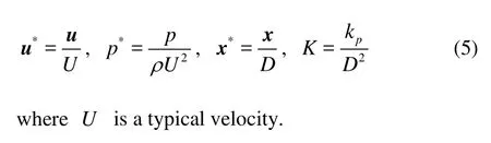
1.1.1 Brinkman system
In view of Eq.(5) and dropping the stars for simplicity, we arrive at the non-dimensional Brinkman system
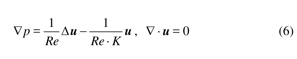
whereRe=ρUD/μis the Reynolds number andKis the Darcy number.
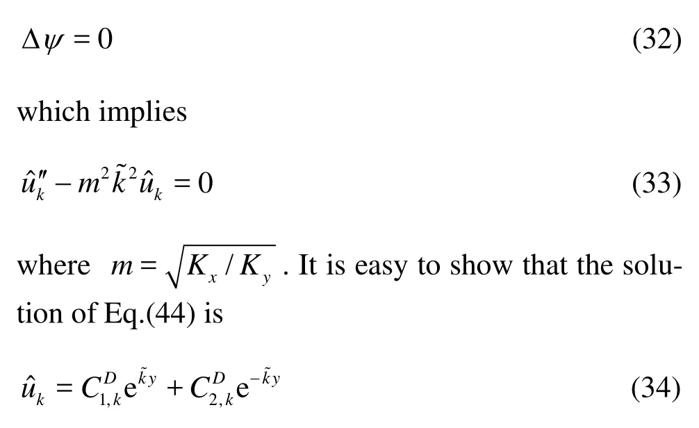
According to the divergence-free condition, there exists a stream functionψsuch that

Taking the curl of the Brinkman equation in Eq.(6), we have, with the help of Eq.(7),
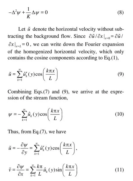
With Eq.(7) in hands, we can solve the Brinkman Eq.(8). For each Fourier mode, with separating variables, we obtain

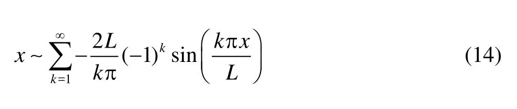
Recall that the Fourier expansions of 1 andxwith respect to sine components read
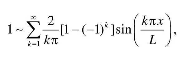
With Eq.(14) in hands, we make the Fourier expansion of the boundary conditions. To match the velocities in the domain, the normal velocity given in Eq.(3) is expanded with respect to its sine component,
1.1.2 Stokes system
The steady state Navier-Stokes equations read

Typically, in the interstitial space, the Reynolds numberRe≪1 so that we can drop the inertia term and thus the Navier-Stokes system reduces to its linear form the Stokes system. To compare the results of the Brinkman system and the Stokes system, we need the solutions of the Stokes equations. We first write down the steady state Stokes system as


1.1.3 Darcy equation
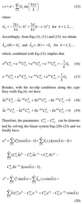
For the non-dimensional number Darcy numberK, heuristically, when it goes to zero, the first term on the right hand side of the Brinkman Eqs.(6) becomes infinitesimally small comparing to the last term (the Darcy-Forchheimer term) and thus it is justified to drop it. The reduced model is the so-called Darcy system,

where we have taken the anisotropy into account. In this paper, we avoid the analytical solution of the anisotropic Brinkman equations, since its expression is very complicated.KxandKyare the longitudinal and transverse permeability in the interstitial space. In the following, we will see that whenKx/Kyis moderate, the isotropic Darcy model can be adopted to approximate the anisotropic one.
Following the same procedure as we have done previously, the corresponding stream function satisfies
Since there are only two free parameters, we just need to impose two boundary conditions: the normal velocities at the capillary wall Eq.(3), which in light of Eq.(34), are expressed as
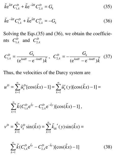

Fig.2 Conceptual domain for the capillary and interstitial space
1.2Coupled Stokes-Darcy model
In the previous section, we concentrate on three different systems to describe the interstitial space, in which we take the Starling formula as the boundary conditions. In this section, we will also take the flow in the capillary into consideration, namely, we will investigate the coupled capillary and interstitial flow. We are interested in the changes of the flows in the interstitial space and the more exact description of the exchange velocity at the interface between the capillary and the interstitial space when the capillaryeffect is considered. According to the symmetry in the vertical direction, we just need to consider the domain [0,L]×[-Hc,Hm], whereHcis the radius of the capillary and 2Hmis the width of the interstitial space (see Fig.2). Now, we begin with the coupled Stokes-Darcy model

whereνt=μi/ρ(i=1,2) is the kinematic viscosity and we denoteβ=ν1/ν2, the subscriptscandmstand for the capillary and the interstitial space, respectively andD(uc)=[∇uc+(∇uc)T]/2 stands for the deformation tensor. Assume that the velocities at the inlet and the outlet of the capillary and the interstitial space are given
We take the same procedure as we have done previously and obtain in the interstitial space
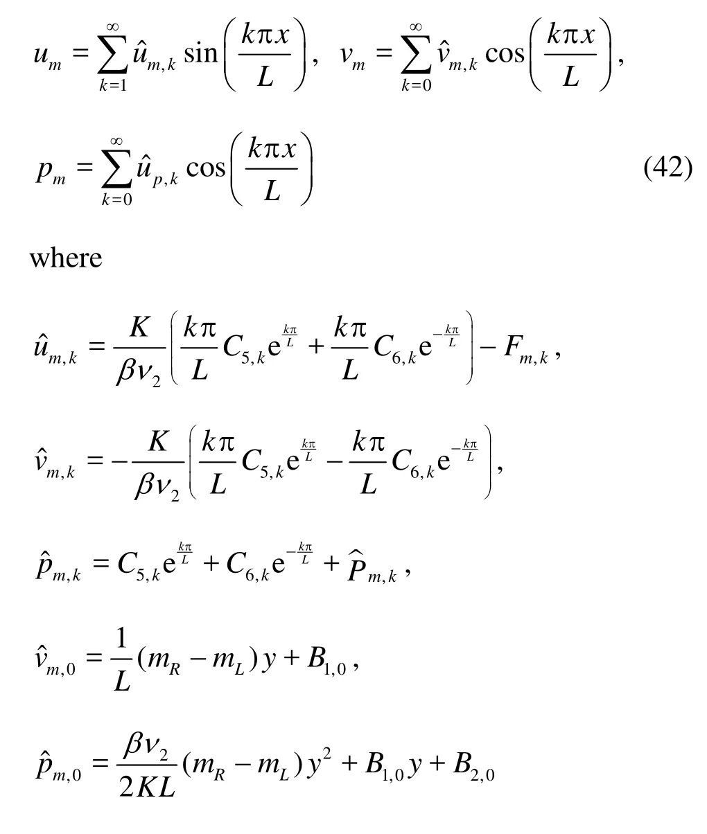
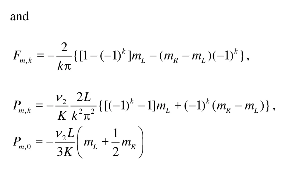
andC5,k,C6,k,B1,0andB2,0are constants to be determined.
On the other hand, in the capillary,

Next, we are going to determine the parameters. For each Fourier modek≠0, there are six free parameters, so that we need the same number of boundary conditions or interface boundary conditions.
Since we assume the total arrangement of the capillaries inydirection is periodic, we assume that there is no flow across the boundary aty=Hm. By the same token, we use the conditions of free slip and no flow penetrating the center axis in the capillary aty=-Hc. At the interface, we use the condition of the continuity of the normal velocity, the continuity of thestress and the no slip condition for the flow in the conduit along the capillary wall[14]. Specifically, these conditions imply

fork=0. By solving the linear algebra system Eq.(44), we obtain the coefficientsC1,k~C6,k, which along with Eq.(45) give the solutions of the coupled Stokes-Darcy model.
2. Results
2.1Analytic analysis of the models
We first investigate some properties from the solutions of the Brinkman model. By solving the linear algebra system Eqs.(16)-(20), we can explicitly write down the analytic solution of the velocities. Yet, the full expression of the coefficientsC1,k~C4,kis quite complicated. Since in most cases, especially, in the interosseous membrane of human, the permeability is small, we are interested in the case where the Darcy number is small. Noticing that in the interstitial fluid, the ratio betweenH, the half width of the domain, andL, the length of the domain, are small, we take the asymptotic expansion of the coefficients Eq.(20) with respect toH/Lfor each Fourier mode when the Fourier modekis not large. That is

From Eq.(46) we observe that
(1) Boundary layers emerge when adopting the Brinkman model. The thickness of the boundary layer is of orderO(1/E), approximatelyO().
(2) Away from the boundary layer, the velocity depends on the strength of the infiltration of the capillary walls as well as the ratio between the length and the height of the domainL/H(since?˜=kπ/L).
(3) Sinceyis small, ek˜yand e-k˜yare close to each other so that their difference is small. Thus the horizontal velocity is larger than the vertical velocity.
Likewise, with the explicit expression of the coefficients in the Darcy system Eq.(37), we can approximate the solution of the Darcy equations with

From Eq.(47) as well as Eq.(46), we have the following observations:
(1) There is also no boundary layer in the solutions of the Darcy model. Settingm=1, i.e., the isotropic case, the solutions of the Darcy model and the Brinkman model (neglecting the boundary layers) are the same, which implies again the Darcy model is a good approximation of the Brinkman model.
(2) Whenkis small, i.e., for several leading order Fourier modes,?˜my≪1 so that
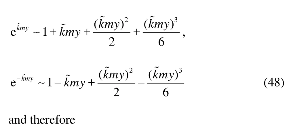

From Eq.(49), it is seen that the leading order term of both the horizontal and vertical velocities derived from Darcy model does not contain the factorm, which implies that the isotropic Darcy model can be used as a good approximation of the anisotropy model whenmis not very large.
Also, from Eq.(49), the leading order term of the horizontal velocity is a constant,

which means that the horizontal outflow is almost uniform independent ofy. Since the solutions of the Darcy system and the Brinkman system are the same when neglecting the boundary layer, this conclusion is also valid for the solution of the Brinkman model.
As to the Stokes system, for a fixedkless than 20, the leading order expression of the horizontal velocity is
From Eq.(50) we observe that:
(1) There is no boundary layer in the expression of the solution derived from the Stokes model.
(2) The velocity at the center axis (y=0) of the Stokes model are 1.5 times as large as that of the Brinkman and Darcy systems and the profiles of the velocity are a parabola.
2.2Some numerical results based on the analytic solutions
We first use the parameters in the interosseous membrane of human as listed in Table 1 in our numerical simulation. The number of terms in the Fourier series to produce the numerical values in the figures is 20.
With these parameters, the Darcy number is,


Table 1 The parameters in the interosseous membrane of human

Fig.3 The horizontal velocity at the center axis of Stokes system and Brinkman system
Thus, the results derived from the Brinkman model and the Darcy model are almost the same. We now compare the results between the Brinkman model and the Stokes model. The horizontal velocities at thecenter axis of both systems are shown in Fig.3. Despite the fact that both velocities have similar profiles, the values are quite distinct. The velocity of the outflow of the Stokes system (2.9360×10⁻⁵m/s) is almost 1.5 times as that of the Brinkman system (1.9596× 10⁻⁵m/s). The maximum velocity at the center axis of the Stokes system is 3.8792×10⁻⁵m/s, which is also 1.5 times as that of the Brinkman system (2.5848× 10⁻⁵m/s). These results are consistent with the analytic conclusion 8. Figure 4 illustrates the horizontal flows at the outlet. It is shown that the outflow of the Stokes model is in parabolic profiles while those of both Brinkman and Darcy models are almost uniform outflows despite the fact that the velocity of the Brinkman model has boundary layers, all of which are again verified by the analysis in the previous section. Figure 5 shows the flow field derived from the Brinkman model, which indicates that the maximum horizontal velocity is at the center axis.

Fig.4 The profiles of the horizontal velocity at the outlet for different systems

Fig.5 The flow field of the Brinkman model
Although the Stokes and Brinkman models appear to be quite disparate under these parameters, our interest is when the Stokes model can be employed as a desirable approximation to the Brinkman model. Heuristically, we know that when the Darcy number is small, the Brinkman equations are reduced to the Darcy equations and when the Darcy number is large, the Brinkman equations approach to the Stokes equations. We might find a quantitative criterion for the adoption of the two simplified models. To this end, we compute the relative error (RE) of the norm of the horizontal velocity with respect to different models at the center axis. From Figure 6 we know that when the Darcy numberDa≥0.2, the Stokes equations approach the Brinkman equations while whenDa≤2×10⁻⁴the Darcy model is an appropriate approximation to the Brinkman model.

Fig.6 The relative error between the results of Stokes and Brinkman models and Darcy and Brinkman models with different Darcy number

Fig.7 The relationship between the outflow at the center axis and the length of the capillary and between the outflow at the center axis and the distance between two neighboring capillaries respectively
Next, we investigate how the length of the capillary and the distance between two neighboring capillaries affect the results. For this purpose, we let the length of the capillary varies from 1 000 μm to 2 000 μm and the vertical distance changes from 40 μm to 60 μm while fixing other parameters. As pointed out, the velocity of the horizontal outflow varies little with respect toy, we just need to consider the flow at the center axis. The results are shown in Fig.7. It is observed that the outflow increases linearly with the increase of the length of the capillary while it decreases with the increase of the distance between the capillaries.

Fig.8 The relative errors of the anisotropic and isotropic Darcy models
Next, we consider the effect of the anisotropy. In solving the Darcy model, we have pointed out that whenKx/Kyand the wave numberkare both not too large, the anisotropy model can be approximated by the isotropic one. Here, we consider the cases of relatively largeKx/Ky. Figure 8 illustrates the relative errors with respect to the horizontal velocities and the vertical velocities between the anisotropic and isotropic Darcy systems. It is shown that whenKx/Kyis small, the numerical results are consistent with the asymptotic analysis so that we can utilize the isotropic Darcy model to approximate the anisotropic one. However, the relative error increases with the increase of the ratio. WhenKx/Ky>20, the error in the vertical direction will be above 10% so we can say that the isotropic approximation is no longer accurate enough forKx/Kylarger than 20. On the other hand, ifKx<Ky, the relative error with respect to the isotropic model is small.
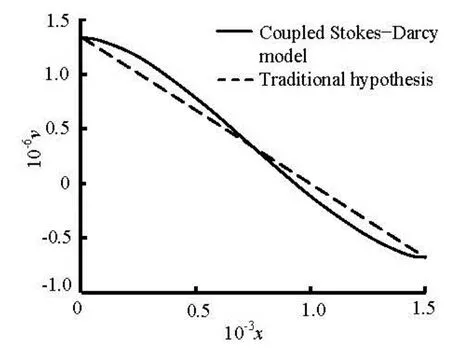
Fig.9 The interface exchange velocity of Stokes-Darcy model compared with the traditional hypothesis
Lastly, we compare the results derived from the coupled Stokes-Darcy model with the single Darcy model. To make the comparison, we adjust the interface exchange velocities to let them equal to each other at the inlet and the outlet. From Fig.9, we observe that the profiles of the interface exchange flows of the coupled Stokes-Darcy model is no longer linear and the influx near the artery and the re-absorption near the vein are both more evident than the Darcy model with the traditional hypothesis that the pressure decreases linearly in the Starling formula. To make a further study of the velocity in the interstitial space, we draw the horizontal velocity at the center axis of the interstitial space as in Fig.10, which shows that the maximum of the velocity in the coupled Stokes-Darcy model is larger and is reached earlier than that in the single Darcy model. This can be explained by the more significant changes at the interface. Besides, we observe that the rates of the outflow are the same, which implies that the total exchange fluxes of the two models are equal. Thus, the approximation by adopting the traditional hypothesis is justified.

Fig.10 The horizontal velocity at the center axis in the interstitial space for coupled Stokes-Darcy model and Darcy model
3. Discussion
Firstly, we compare our results with our previous numerical simulation results[6]. It shows that our analytic solutions agree with our simulation solutions obtained by Fluent software.
Our results demonstrate the difference between the solutions of the Stokes, Brinkman and Darcy equations. Typically, since the hydraulic permeabilitykpin the interosseous membrane is small, we recommend the Darcy system to approximate the Brinkman model. Otherwise, the Stokes equations can be regarded as a good approximation to describe the fluid flow in the interstitial space for relatively largekp. The maximum relative error between the Darcy and Stokes systems is 50% and therefore improper use of the models will bring about a significant inaccuracy. To decide which model is more suitable, the Darcy number is animportant factor, as seen from the criterion deduced from Fig.6. Chen’s results show the parallel arrangement of collagen fibrils will certainly lead to the anisotropic permeability property in the tissue[6]. However, most models that describe the continuum tissue employ the isotropic assumption[5]. But, on the one hand, it is difficult to deduce the analytic solutions of the Brinkman equation with anisotropic permeability and, on the other hand, it is almost impossible to determine the ratio of the longitudinal permeabilityKxto the transverse permeabilityKy(Kx/Ky). Fortunately, in light of the analytic expression of the Darcy equation with anisotropic permeability, we find that the relative error between the anisotropic and isotropic Darcy models is small ifKx/Kyis not very large, which is especially true forKx/Ky<1. The critical value of this ratio isKx/Ky=20, above that ratio, a relative error in the vertical velocity more than 10% will occur. Yet, we have to point out that, the influence of the anisotropy also depends on the geometry of the interstitial space according to the asymptotic expression (49), which shows that the shorter the capillaries are or the wider their distance is, the more important the influence will be. Chen’s simulations show thatKxis definitely larger thanKyand the maximum value ofKx/Kycan be up to 50[6], which implies that the anisotropic permeability must be considered.
The coupled Stokes-Darcy model shows that the profiles of the interface exchange flows are no longer linear as some models suggest[8]and the re-absorption near the vein is more evident than in the Darcy model. Yet, the rate of the outflow scarcely changes so that the traditional assumption of adopting the exchange flows with a linear profile can be acceptable. Though the nonlinear boundary condition only slightly affects the interstitial fluid flow (See Fig.10), it may be important for the mechanism of some cardiovascular diseases such as atherosclerotic. For example, Tarbell studied the biochemical responses of Smooth Muscle Cells (SMCs) to the interstitial fluid through blood vessel walls[9]. Hayward found that with appropriate length and branching degree of the capillary-like structures, the permeability flow value reaches the maximum,when the capillary wall is 10 μm/min to 20 μm/min.
The interaction between the tissue fluid and the blood flow is an important issue in the interstitial fluid flow. The arrangement of capillaries and the permeability velocity will affect the flow velocity greatly. The velocity field shows that the direction of the interstitial fluid flow is parallel to the orientation of capillaries. When there is no inlet flow, the maximum velocity in the Brinkman model is 2.5848×10⁻⁵m/s, and the velocity at the outlet is 1.9596×10⁻⁵m/s (0.0012 m/min) through the two parallel capillaries. If the fluid from the capillaries is not absorbed by lymphatic, it flows downstream. As our analytic solutions show, the flow field is the superposition of two parts: the inlet flow and the flow field without the inlet flow (as in our model). When the fluid flows downstream, it will be accelerated through another group of parallel capillaries. After several groups of capillaries, the interstitial fluid velocity can reach a magnitude in order of cm/min. It is possible that the long interstitial tissue channels observed by Casley-Smith with the electro microscope are in fact the interstitial fluid flow[6]. The tracer (Gd-DTPA) injected into the acupoint travels with the interstitial fluid flow, therefore, their observations of the flow different from the blood and lymph flow should reflect the interstitial fluid flow[7].
Though the numerical simulation shows that the flow velocity is small (10–5m/s), it is still important to the cells’ physiology. Only under the flow environment, the lymphocyte can organize into a functional lymphatic network. The lymphatic development direction is the same as the interstitial fluid flow, and the decreasing flow velocity will restrain the lymphatic development[16]. It is shown that 12.5 μm/s-5.6 μm/s is the best velocity range for cell alignment and proliferating[17]. Anisotropy is also an important factor. Previous computational studies show that when the tissue is modeled as spatially homogenous, the fluid flow stimulus does not significantly affect the tissue differentiation[15]. However, as soon as the spatial heterogeneity in material properties is developed, the interstitial fluid velocity will be a determining factor[6]. The mechanism of the effect of the interstitial flow on the cell bioactivities is unknown. It is generally believed that the sheer stress induced by the flow is mainly responsible. We found that thein vitromast cell is activated by the stretch stress[6]and the mast cellsin situcan be activated by the flow[6]. These experimental results suggest that the interstitial fluid flow is important in physiology.
[1] COWIN STEPHEN. Bone Mechanics Handbook[M]. 2nd edition, Boca Raton, USA: CRC press, 2001, 1-29.
[2] TARBELL J. M., WEINBAUM S. and KAMM R. D. Cellular fluid mechanics and mechanotransduction[J]. Annals of Biomedical Engineering, 2005, 33(12): 1719-1723.
[3] NG C. P., SWARTZ M. A. Fibroblast alignment under interstitial fluid flow using a novel 3-D tissue culture model[J]. American Journal of Physiology-Heart Circulatory Physiology, 2003, 284(5): 1771-1777.
[4] HAYWARD L. N. M., MORGAN E. F. Assessment of a mechano-regulation theory of skeletal tissue differentiation in an in vivo model of mechanically induced cartilage formation[J]. Biomechanics and Modeling inMechanobiology, 2009, 8(6): 447-455.
[5] PEDERSEN J. A., BOSCHETTI F. and SWARTZ M. A. Effects of extracellular fiber architecture on cell membrane shear stress in a 3D fibrous matrix[J]. Journal of Biomechanics, 2007, 40(7): 1484-1492.
[6] YAO Wei, DING Guang-hong. Interstitial fluid flow: simulation of mech6nical environment of cells in the interosseous membrane[J]. Acta Mechanica Sinica, 2011, 27(4): 602-610.
[7] LI H. Y., YANG J. F. and CHEN M. Visualized regional hypodermic migration channels of interstitial fluid in human beings: Are these ancient meridians?[J]. The Journal of Alternative and Complementary Medicine, 2008, 14(6): 621-628.
[8] ZHANG Di, YAO Wei and DING Guang-hong et al. A fluid mechanics model of tissue fluid flow in limb connective tissue-a mechanism of acupuncture signal transmission[J]. Journal of Hydrodynamics, 2009, 21(5): 675-684.
[9] SHIGERU T., TARBELL J. M. Flow through internal elastic lamina affects shear stress on smooth muscle cells (3D simulations)[J]. American Journal of Physiology-heart and Circulatory Physiology, 2002, 282(2): 576-584.
[10] FENG J., WEINBAUM S. Flow through an orifice in a fibrous medium with application to fenestral pores in biological tissue[J]. Chemical Engineering Science, 2001, 56(18): 5255-5268.
[11] RÉMOND A., NAILI S. and LEMAIRE T. Interstitial fluid flow in the osteon with spatial gradients of mechanical properties: A finite element study[J]. Biomechanics and modeling in Mechanobiology, 2008, 7(6): 487-495.
[12] GALLEY S. A., MICHALEK D. J. and DONAHUE S. W. A fatigue microcrack alters fluid velocities in a computational model of interstitial fluid flow in cortical bone[J]. Journal of Biomechanics, 2006, 39(11): 2026-2033.
[13] KEENER J., SNEYD J. Mathematical physiology[M]. Second Edition, New York, USA: Springer-Verlag 2009, 547.
[14] DISCACCIATI M., QUARTERONI A. Analysis of a domain decomposition method for the coupling of the Stokes and Darcy equations[C]. Numerical Mathematics and Advanced Applications. Milan, Italy, 2003, 3-20.
[15] EPARI D. R., TAYLOR W. R. and HELLER M. et al. Mechanical conditions in the initial phase of bone healing[J]. Clinical Biomechanics, 2006, 21(6): 646-655.
[16] NG C. P., HELM C. L. E. and SWARTZ M. A. Interstitial flow differentially stimulates blood and lymphatic endothelial cell morphogenesis in vitro[J]. Microvascular Research, 2004, 68(3): 258-264.
[17] NG C. P., SWARTZ M. A. Mechanisms of interstitial flow-induced remodeling of fibroblast-collagen cultures[J]. Annals of Biomedical Engineering, 2006, 34(3): 446-454.
10.1016/S1001-6058(13)60413-8
* Project supported by the National Natural Science Foundation of China (Grant No. 11202053) the Shanghai Science Foundation (Grant No. 12ZR1401100) and the National Key Basic Research Program of China (973 Program, Grant No. 2012CB518502).
Biography: YAO Wei (1973-), Female, Ph. D.,
Associate Professor
杂志排行

水动力学研究与进展 B辑的其它文章
- A one-dimensional polynomial chaos method in CFD–Based uncertainty quantification for ship hydrodynamic performance*
- Numerical analysis of cavitation within slanted axial-flow pump*
- Numerical simulation of hydro-elastic problems with smoothed particle hydrodynamics method*
- Experimental study of shell side flow-induced vibration of conical spiral tube bundle*
- A streamline approach for identification of the flowing and stagnant zones for five-spot well patterns in low permeability reservoirs*
- Theoretical analysis and experimental study of oxygen transfer under regular and non-breaking waves*