A one-dimensional polynomial chaos method in CFD–Based uncertainty quantification for ship hydrodynamic performance*

HE Wei (贺伟)

School of Naval Architecture, Ocean and Civil Engineering, Shanghai Jiao Tong University, Shanghai, China

IIHR-Hydroscience and Engineering, The University of Iowa, Iowa City, USA, E-mail: helloweihe@gmail.com

DIEZ Matteo

IIHR-Hydroscience and Engineering, The University of Iowa, Iowa City, USA

CNR-INSEAN, National Research Council-Maritime Research Centre, Rome, Italy

CAMPANA Emilio Fortunato

CNR-INSEAN, National Research Council, Maritime Research Centre, Rome, Italy

STERN Frederick

IIHR-Hydroscience and Engineering, The University of Iowa, Iowa City, USA

ZOU Zao-jian (邹早建)

School of Naval Architecture, Ocean and Civil Engineering and State Key Laboratory of Ocean Engineering, Shanghai Jiao Tong University, Shanghai, China

(Received January 15, 2013, Revised April 7, 2013)

A one-dimensional polynomial chaos method in CFD–Based uncertainty quantification for ship hydrodynamic performance*

HE Wei (贺伟)

School of Naval Architecture, Ocean and Civil Engineering, Shanghai Jiao Tong University, Shanghai, China

IIHR-Hydroscience and Engineering, The University of Iowa, Iowa City, USA, E-mail: helloweihe@gmail.com

DIEZ Matteo

IIHR-Hydroscience and Engineering, The University of Iowa, Iowa City, USA

CNR-INSEAN, National Research Council-Maritime Research Centre, Rome, Italy

CAMPANA Emilio Fortunato

CNR-INSEAN, National Research Council, Maritime Research Centre, Rome, Italy

STERN Frederick

IIHR-Hydroscience and Engineering, The University of Iowa, Iowa City, USA

ZOU Zao-jian (邹早建)

School of Naval Architecture, Ocean and Civil Engineering and State Key Laboratory of Ocean Engineering, Shanghai Jiao Tong University, Shanghai, China

(Received January 15, 2013, Revised April 7, 2013)

A one-dimensional non-intrusive Polynomial Chaos (PC) method is applied in Uncertainty Quantification (UQ) studies for CFD–based ship performances simulations. The uncertainty properties of Expected Value (EV) and Standard Deviation (SD) are evaluated by solving the PC coefficients from a linear system of algebraic equations. The one-dimensional PC with the Legendre polynomials is applied to: (1) stochastic input domain and (2) Cumulative Distribution Function (CDF) image domain, allowing for more flexibility. The PC method is validated with the Monte-Carlo benchmark results in several high-fidelity, CFD-based, ship UQ problems, evaluating the geometrical, operational and environmental uncertainties for the Delft Catamaran 372. Convergence is studied versus PC orderPfor both EV and SD, showing that high order PC is not necessary for present applications. Comparison is carried out for PC with/without the least square minimization when solving the PC coefficients. The least square minimization, using larger number of CFD samples, is recommended for current test cases. The study shows the potentials of PC method in Robust Design Optimization (RDO) and Reliability-Based Design Optimization (RBDO) of ship hydrodynamic performances.

Uncertainty Quantification (UQ), Polynomial Chaos (PC) method, Legendre polynomials, ship design

Introduction

In engineering application, Robust Design Optimization (RDO) and Reliability-Based Design Optimization (RBDO) are receiving more and more interest, considering the uncertainties on design objectives, inherited from input uncertainties, e.g., operational, environmental and manufactural uncertainty[1]. As an essential part of RDO and RBDO, stochastic Uncertainty Quantification (UQ) studies the effects of uncertain input on the relevant output parameters, namely optimization objectives and constraints. The UQ method focuses on assessing the stochastic properties of simulation outputs, including Expected Value (EV), Standard Deviation (SD), Probability Density Function (PDF) and Cumulative Distribution Function (CDF).

Several methods have been used to propagate the uncertainty in stochastic applications, such as the Monte-Carlo (MC) method, interval analysis, sensiti-vity derivatives, and moment methods. The MC method, which is statistical, non-intrusive and easy to use, is a powerful tool in UQ study. Nevertheless, the MC method requires a larger number of samples and becomes very expensive in high-fidelity simulations, especially in RDO and RBDO. Using metamodels (“model of the model”) could reduce the number of required deterministic simulations by constructing approximations of the analysis code outputs. Using a set of known data (computational or experimental data), a metamodel can fit the data to some simple or inexpensive functions, providing fast analysis for uncertainty space exploration and describing the nonlinear relationship between the input and output variables. There are various options of metamodel techniques, such as the Response Surface (RS), Neural Networks (NN), Support Vector Machine (SVM) and Kriging. Simpson et al.[2,3]reviewed these techniques and summarized their characteristics and appropriate uses.

Quadrature formulas can also be used for UQ, e.g., numerical integration methods like trapezoidal and Simpson’s rules, Gaussian quadrature and Polynomial Chaos (PC) method. Mousaviraad et al.[4]tested and summarized several integration methods in previous UQ studies, including the polynomial chaos and Gaussian quadrature. Gaussian quadrature requires distinctive items according to the selected formula, while PC is more flexible to use any samples. PC was originally introduced by Wiener[5]and is an integral approach to propagate the stochastic properties in UQ study. As a spectral method, PC projects the variables of the problem onto a stochastic space spanned by a set of orthogonal polynomials, e.g., the Hermite polynomials, Laguerre polynomials, Jacobi polynomials and Legendre polynomials. UQ properties, EV and SD, are derived from the coefficients of PC expansions. In fluid mechanics, Mathelin et al.[6]studied the uncertainty propagation for turbulent compressible nozzle flow. Hosder et al.[7]studied non-intrusive PC method for uncertainty quantification in CFD simulations. Weaver and Alexeenko[8]studied flow field uncertainty for hypersonic CFD simulations. Mousaviraad et al.[4]studied the PC method for a 2-D airfoil NACA0012 at the stochastic Reynolds Number (Re).

The present work studies the PC method in CFD–based UQ of ship resistance and motions in variable geometry, speed and waves for the Delft Catamaran 372. Test data are taken from earlier MC studies. PC is carried out in both the stochastic input domain and the CDF-image domain. The convergence versus the orderPis investigated with/without the least square minimization in solving PC parameters, and the accuracy is validated versus the MC benchmark using CFD simulations. Proper orderPand PC formulations are recommended. PC gives the polynomial representation of the response function as a metamodel. This means that PC can also be used to study the PDFs and CDFs for output variables using the MC approach. Current study focuses on the PC capability of assessing EV and SD, leaving distribution studies for future work.

1. The PC methodology

UQ evaluates the stochastic effects of a random inputξon a random outputu, including EV, SD, PDF and CDF. Bothξanducould be multi-dimensional. The focus is here on EV and SD, given by

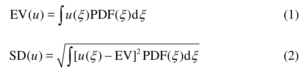
The concept of PC decomposes a random variable into separable deterministic and stochastic components. For example, for stochastic variableu, such as the total resistance of a ship, its functional dependence is typically expressed in terms of a series[9]

whereξis then-dimensional stochastic input variable,u(ξ) is the random output variable,αiis the socalled deterministic component andΨi(ξ) is the stochastic component, corresponding to thei-th mode.

In Eq.(3),αicould be treated as the amplitude of thei-th fluctuation. For a multi-dimensional variableξ, the number of modes equalsP+1=(n+p)!/n!p!, which is a function of the order of PC(p) and the stochastic input dimension (n). In one-dimensional UQ problems,P=p. The stochastic basis functionsΨi(ξ), used in PC expansions, are selected as orthogonal polynomials, assuming an inner product with weight equal to the PDF of the random inputξ.

1.1Orthogonal polynomials

In a system of orthogonal polynomials (assuming single-valued functions), we denote a set of {Ψi}?, whereΨiis a polynomial of degreei. The polynomials are deemed orthogonal in the sense that the inner productΨi,Ψjvanishes asi≠j.

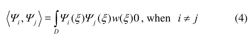
wherew()ξis a positive weight function.

Using constantw(ξ)=wwithinξ∈[-1,1], the first eleven one-dimensional Legendre polynomials are given in Table 1.

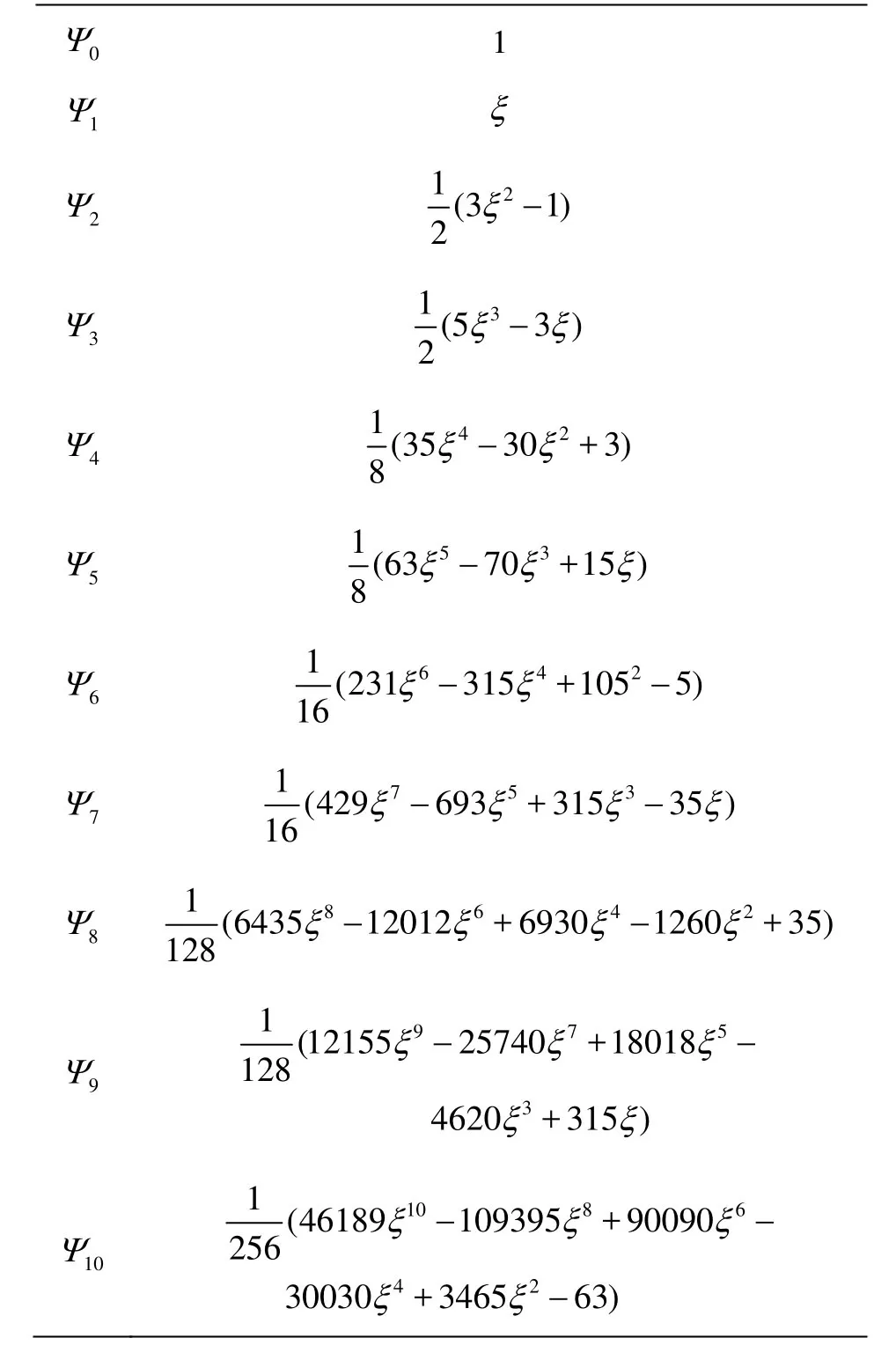
Table 1 The first eleven one-dimensional Legendre polynomials

The inner products are given by

1.2one-dimensional PC in input variable domain (ξ domain)

Assume that the random variableξfollows a uniform distribution within -1＜ξ＜1, then the PDF of the random variableξis PDF(ξ)=1/2, with -1＜ξ＜1. The stochastic properties of the output variableuin Eqs.(1) and (2) are expressed as

Combining Eq.(3) and Eq.(4), from Eqs.(6) and (7) we have

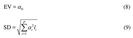
For a given one-dimensional PC expansion of orderP, if we chooseNitemsξi(N≥P+1) and get the deterministic solutionsui, a linear system can be given as

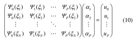
All deterministic componentsiαcan be determined from the linear system of Eq.(10). EV and SD can be assessed from Eqs.(8) and (9).

It may be noted that orthogonal polynomials have to be redefined according to the given PDF (weight function) and input range. For example, the Hermite polynomials are used with Gaussian distributions, the Laguerre polynomials with the Gamma distributions and the Jacobi polynomials with the Beta distributions, etc.[9].

1.3one-dimensional PC in probability domain (C domain)

If the inputξfollows an arbitrary (non-standard) distribution, it is not trivial to get the corresponding orthogonal polynomials. One easy solution is redefining the PC expansions in the CDF-image domain (Cdomain) as follows:

Define a new variableC,

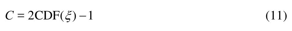
Since CDF is a monotone function, Eq.(11) is equivalent to

where CFD()ξis the cumulative distribution function of the stochastic variableξ.

Equations (1) and (2) become

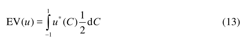
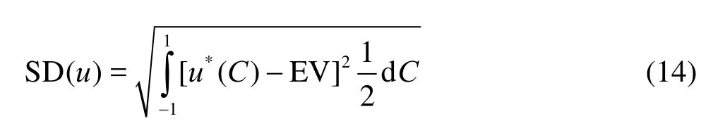
Equations (13) and (14) represent the assessment of EV and SD, expressed in the CDF-image domain. The Legendre polynomials can be used for the orthogonal PC expansions.

2. Convergence and validation

The convergence study uses the concept of verification study in CFD simulation[4]. For a single triplet convergence study, the PC order for large, medium and smallPvalues are denoted as1P,2P,3P, respectively, with a systematic decrease

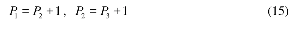
The corresponding EV and SD estimated from PC ofPare used to determine the convergence ratio. For EV, for example, we have

The validation is carried out for EV and SD, using the benchmark MC data with the related validation uncertainty.

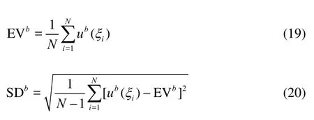
The benchmark values (denoted by superscriptb) are evaluated as

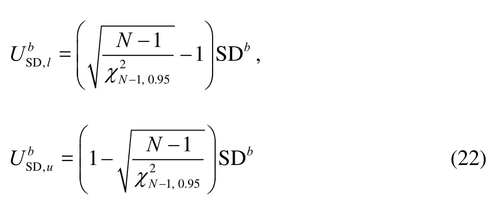
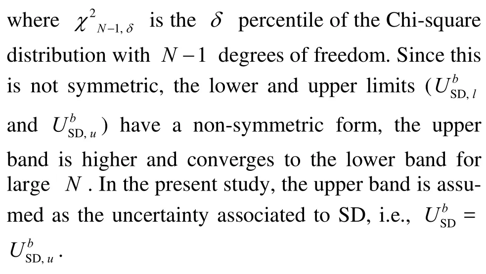
Validation uncertaintiesUandUare estimated at 95% level of confidence as follows

wheretN-1,0.95is the Studentt-distribution withN-1 degrees of freedom at 95% confidence interval, which approximately equals 2 for largeN. For SD, it follows that

The comparison errors for EV and SD are defined as

3. Applications of pc method in one-dimensional UQ problems

In the present study, the non-intrusive PC approach is tested on three CFD-based UQ studies for ship hydrodynamic performances, quantifying the UQ properties of ship resistance and motions inherited from geometric, operational and environmental uncertainties for the Delft Catamaran 372 in calm water and regular waves. The Delft Catamaran 372 has been selected as an international benchmark for research programs in CFD (Office of Naval Research, Naval International Cooperative Opportunities in Science and Technology Programs and NATO Advanced Vehicle Technology Activities), including the waterjet propelled optimization[10], interference[11,12]and seakeeping[13]studies, and stochastic UQ and optimization[1].

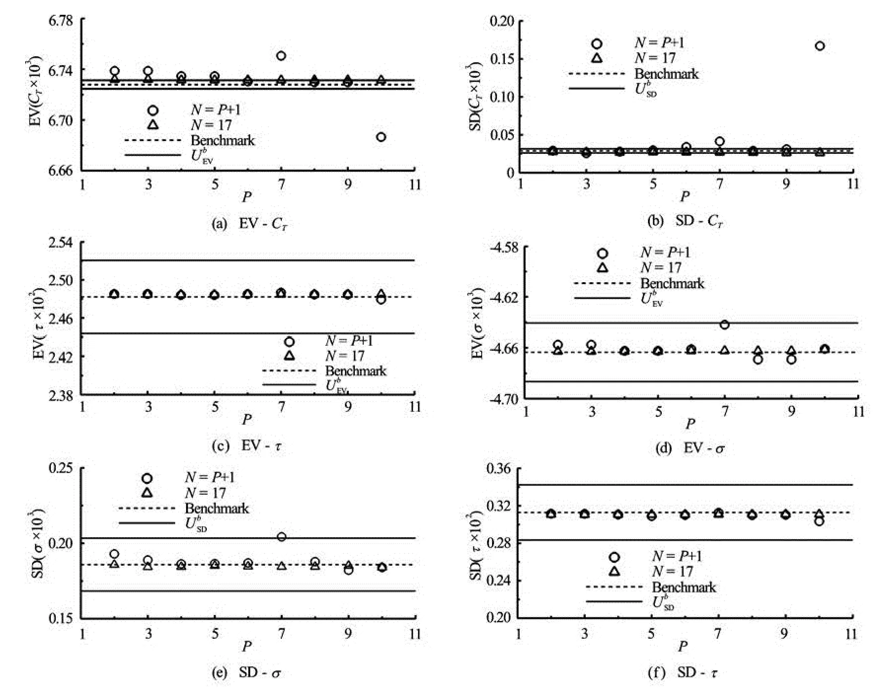
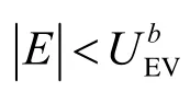
Fig.1 Convergence of EV and SD for (a), (d)CT, (b), (e)σand (c), (f)τvariable geometry

The Benchmark items used for EVband SDbare obtained using the MC method associated with the Latin Hyper Cube (LHS) sampling. CFD Ship-Iowa V4.5 is used for the deterministic simulations with the hybridk-ε/k-ωturbulence model and singlephase level set free-surface model. Numerical methods include the advanced iterative solvers, second- and higher-order finite difference schemes with conservative formulations, parallelization based on a domain decomposition approach using the message-passing interface, and dynamic overset grids for 6-DOF large-amplitude motions. The fluid flow equations are solved in an earth-fixed inertial reference system, while the rigid body equations are solved in the ship system. All the simulations ran on an HPC cluster.

Nsamples are picked from the benchmark data to formulate the linear system of Eq.(10).Nis chosen as (1) equal toP+1 or (2) constant and equal to 17. AsN＞P+1, Eq.(10) is solved by least square minimization.

3.1Variable geometry

This one-dimensional UQ problem studies the effects of the geometric uncertainty on calm water total resistance coefficientC1=RT/(0.5ρU2S) (whereRTis the total resistance,Uthe ship speed,ρthe water density, andSthe static wetted hull surface), non-dimensional sinkageσ=sinkage/Land trimτin radians, whereLis the ship length. The ship is advancing at the Froude NumberFr=0.5. The geometry (G) is defined as a linear interpolation from the original design (G0) to a modified design (G1), i.e.,G=(1-α)G0+αG1. In this case, the geometry modifications represent the first principal direction of the Karhunen-Loève expansion of a multi-dimensional optimization research space, as presented in Ref.[14]. The geometric variableαfollows a uniform distribution within [0,1]. Accordingly, it is PDF(α)=1.

The benchmark MC study consists of 257 LHS items with EVb=6.728×10-3, -4.664×10-3and 2.482×10-2, SDb=0.029×10-3, 0.186×10-3, and 0.313×10-2,U?=0.05, 0.49 and 1.55%EVb,U= 9.43, 9.43 and 9.43%SDb, forCT,σandτ, respectively.

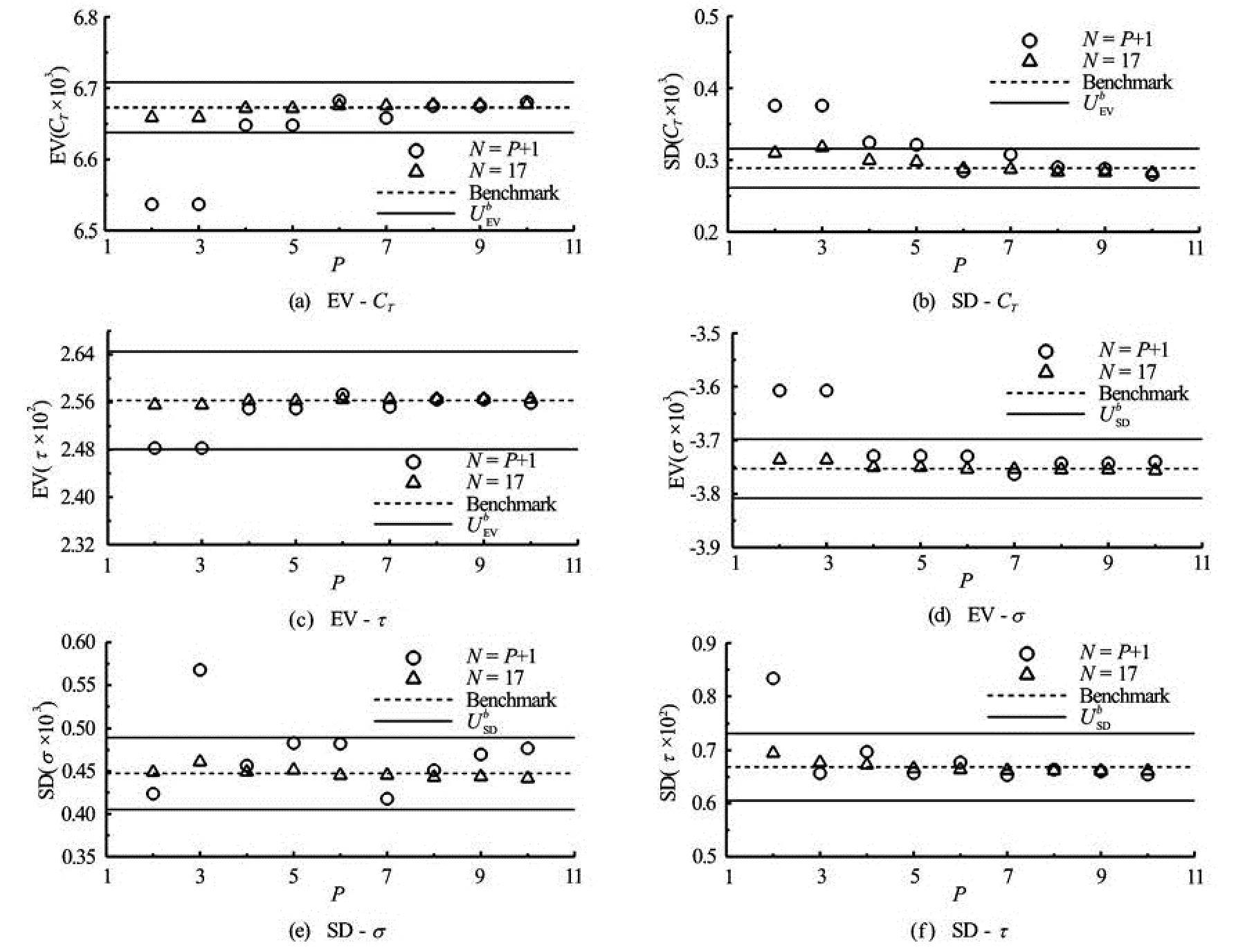
Fig.2 Convergence of EV and SD for (a), (d)CT, (b), (e)σand (c), (f)τvariableFr

PC is carried out in theξdomain, usingNLHS items from the benchmark data, withPincreasing from 2 to 10. The convergence versusPis studied for bothN=P+1 andN=17. Figure 1 shows the EV and SD versusPforCT,σandτ, respectively.N=17 shows better convergence thanN=P+1 for both EV and SD, and has less fluctuation (ε12) and errors thanN=P+1. WhenN=P+1, the error of EV is smaller than 1% for all output variables, and gets larger at high order for variableCT.Eof SD is larger than EV. For SD ofCTatP=10,E= 482%SDb,R=65,ε12=81%SD1, showing divergence of the results. Most of the PC estimations are validated whenN=P+1, except forCTatP=10. WhenN=17, the error of EV is at/under 0.1% level andε12is smaller than 0.01%, the error of SD is under 10% level andε12is less than 1%. PC shows good convergence status. All PC estimations are validated usingN=17. High orderPcannot guarantee the best convergence and errors. The most suitable order is found to be between 4 and 8.

3.2Variable speed(Fr)

This one-dimensional UQ problem studies the uncertainties ofCT,σandτunder stochastic speed, defined byFr. The stochasticFris described by a normal distribution with the mean valueμ=0.5 and the standard deviationσ=0.05 and is truncated within 95% confidence interval

where [0.402,0.598] is the truncation interval.

The benchmark MC study consists of 257 LHS deterministic items with EVb=6.673×10-3, -3.753× 10-3and 2.563×10-2, SDb=0.288×10-3, 0.447×10-3and 0.668×10-2,U?=0.5, 1.5 and 3.2%EVb,U= 9.43, 9.43 and 9.43%SDb, forCT,σandτ, respectively.

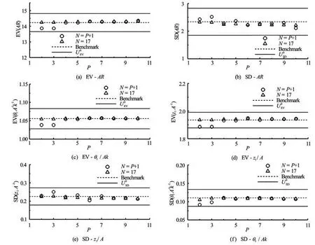
Fig.3 Convergence of EV and SD for (a), (d)AR, (b), (e)z1/Aand (c), (f)θ1/Akvariableλ/L

Since the normal distribution is truncated within the 95% confidence interval, the Hermite polynomials are not suitable to formulate the PC expansions in theξdomain (since not orthogonal, due to truncation). PC is carried out in theCdomain, associated to Legendre polynomials. The orderPtakes from 2 to 10, andNis chosen as (1)N=P+1 or (2)N=17. Figure 2 shows the EV and SD versusPforCT,σandτ, respectively. UsingN=P+1,ε12is between 0 and 1% for EV. SD shows divergence and largeε12, e.g., SD ofCThas monotonic divergence andε12= 13% at the 6th order. AsN=17,Eof EV is smaller than 1%,ε12of EV is under 0.05%.ε12is around 1% for SD. Convergence is much better forN=17 than forN=P+1. Low order PC expansions, usingN=P+1, do not achieve validation. Through investigating the validation errors, it is found the proper orderPis different forCT,σandτ. Lower and higher order PC do not achieve high accuracy (especially usingN=P+1).

3.3Variable regular head waves

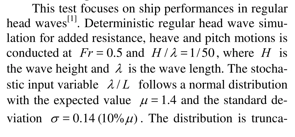
The benchmark MC data consist of 65 LHS items, with EVb=14.23, 1.934 and 1.056, SDb=2.34, 0.226 and 0.110,UbEV=4.1, 2.9 and 2.6%EVb,USbD=9.43, 9.43 and 9.43%SDbforAR,z1/Aandθ1/Ak, respectively.

PC is carried out in theCdomain withPincreasing from 2 to 10. The convergence versusPis studied using (1)N=P+1 and (2)N=17. Figure 3 shows EV and SD versus the PC orderPforAR,z1/Aandθ1/Ak, respectively. AsP＞4,N=P+1 shows similar accuracy asN=17 for all variables ex-cept SD ofAR. The effects of orderPon EV and SD estimations are large usingN=P+1. Specifically, usingN=P+1,E＜1% for EV andE＜10% for SD, while usingN=17,E＜0.5% for EV andE＜0.5% for SD. UsingN=17 yields on averageε12＜1% and better convergence versusPthan usingN=P+1. All PC estimations are validated. UsingN=17 yields better performance than usingN=P+1. However,N=17 does not improve significantly SD estimation using low order PC expansions.

4. Concluding remarks

A one-dimensional PC method has been applied using (1) the stochastic input domain and (2) the CDF-image domain. The PC method has been tested on three UQ problems assessing CFD-based ship hydrodynamic performance, for stochastic geometry, speed and waves. Convergence and validation versus the Monte-Carlo benchmark data have been demonstrated.

The most suitable PC expansion-orderPis found to be problem-dependent. Generally, the current problems suggest the PC order to be in the interval 4≤P≤8.

The least square minimization (N＞P+1) usually gives better convergence and reduces the comparison error, and is recommended for current applications. As a drawback, it should be noted that the least square minimization requires a larger number of CFD simulations.

PC requires small number of deterministic items, and is easy to use in one-dimensional UQ study when input PDF (or CDF) is known. Extension of the current work includes using PC expansions as metamodels to assess output distributions.The PC method could be an option to evaluate EV, SD and distributions in RDO and RBDO in ship design studies.

Acknowledgment

This work was supported by the Office of Naval Research (Grant No. N000141110237), the NICOP (Grant No. N629091117011), under the admission of Dr. Kim Ki-Han. The research was conducted in collaboration with NATO AVT-191: Application of Sensitivity Analysis and Uncertainty Quantification to Military Vehicle Design.

[1] HE W., DIEZ M. and PERI D. et al. URANS study of delft catamaran total/added resistance, motions and slamming loads in head sea including irregular wave and uncertainty quantification for variable regular wave and geometry[C]. Proceedings of the 29th Symposium on Naval Hydrodynamics. Gothenburg, Sweden, 2012.

[2] JIN R., CHEN W. and SIMPSON T. W. Comparative studies of metamodelling techniques under multiple modeling criteria[J]. Structural and Multidisciplinary Optimization, 2001, 23(1): 1-13.

[3] SIMPSON T. W., PEPLINSKI J. D. and KOCH P. N. et al. Metamodels for computer-based engineering design: Survey and recommendations[J]. Engineering with Computers, 2001, 17(2): 129-150.

[4] MOUSAVIRAAD S. M., HE W. and DIEZ M. et al. Framework for convergence and validation of stochastic uncertainty quantification and relationship to deterministic verification and validation[J]. International Journal for Uncertainty Quantification, 2012, 3: 371-395.

[5] WIENER N. The homogeneous chaos[J]. American Journal of Mathematics, 1938, 60(4): 897-936.

[6] MATHELIN L., HUSSAINI M. Y. and ZANG T. A. et al. Uncertainty propagation for a turbulent, compressible nozzle flow using stochastic methods[J]. AIAA Journal, 2004, 42(8): 1669-1676.

[7] HOSDER S., WALTERS R. W. and PEREZ R. A nonintrusive polynomial chaos method for uncertainty propagation in CFD simulations[C]. Proceeding of the 44th AIAA Aerospace Science Meeting. Reno, Nevada, 2006.

[8] WEAVER A. B., ALEXEENKO A. A. Flowfield uncertainty analysis for hypersonic CFD simulations[C]. 48th AIAA Aerospace Sciences Meeting Including the New Horizons Forum and Aerospace Exposition. Orlando, Florida, USA, 2010.

[9] Le MAÎTRE O. P., KNIO O. M. Spectral methods for uncertainty quantification: with applications to computational fluid dynamics[M]. Dordrecht, Heidelberg, London and New York: Springer, 2010.

[10] KANDASAMY M., HE W. and TAKAI T. et al. Optimization of waterjet propelled high speed ships-JHSS and Delft Catamaran[C]. 11th International Conference on Fast Sea Transportation (FAST2011). Honolulu, Hawaii, USA, 2011.

[11] BROGLIA R., BOUSCASSE B. and JACOB B. et al. Calm water and seakeeping investigation for a fast catamaran[C]. 11th International Conference on Fast Sea Transportation (FAST2011). Honolulu, Hawaii, USA, 2011.

[12] BROGLIA R., ZAGHI S. and MASCIO A. D. Numerical simulation of interference effects for a high-speed catamaran[J]. Journal of Marine Science and Technology, 2011, 16(3): 254-269.

[13] CASTIGLIONE T., STERN F. and BOVA S. et al. Numerical investigation of the seakeeping behavior of a catamaran advancing in regular head waves[J]. Ocean Engineering, 2011, 38(16): 1806-1822.

[14] DIEZ M., CAMPANA E. F. and STERN F. Karhunen-Loève expansion for assessing stochastic subspaces in geometry optimization and geometric uncertainty quantification[R]. IIHR Technical Report No. 481, 2012.

10.1016/S1001-6058(13)60410-2

* Project supported by the National Natural Science Foundation of China (Grant No. 50979060).

Biography: HE Wei (1985-), Male, Ph. D. Candidate

ZOU Zao-jian,

E-mail: zjzou@sjtu.edu.cn