Numerical analysis of cavitation within slanted axial-flow pump*
2013-06-01ZHANGRui张睿
ZHANG Rui (张睿)
Shanghai Institute of Applied Mathematics and Mechanics, Shanghai University, Shanghai 200072, China,
E-mail: gulie1984@163.com
CHEN Hong-xun (陈红勋)
Shanghai Institute of Applied Mathematics and Mechanics and Shanghai Key Laboratory of Mechanics in Energy Engineering, Shanghai University, Shanghai 200072, China
(Received November 20, 2012, Revised May 2, 2013)
Numerical analysis of cavitation within slanted axial-flow pump*
ZHANG Rui (张睿)
Shanghai Institute of Applied Mathematics and Mechanics, Shanghai University, Shanghai 200072, China,
E-mail: gulie1984@163.com
CHEN Hong-xun (陈红勋)
Shanghai Institute of Applied Mathematics and Mechanics and Shanghai Key Laboratory of Mechanics in Energy Engineering, Shanghai University, Shanghai 200072, China
(Received November 20, 2012, Revised May 2, 2013)
In this paper, the cavitating flow within a slanted axial-flow pump is numerically researched. The hydraulic and cavitation performance of the slanted axial-flow pump under different operation conditions are estimated. Compared with the experimental hydraulic performance curves, the numerical results show that the filter-based model is better than the standardk-εmodel to predict the parameters of hydraulic performance. In cavitation simulation, compared with the experimental results, the proposed numerical method has good predicting ability. Under different cavitation conditions, the internal cavitating flow fields within slanted axial-flow pump are investigated. Compared with flow visualization results, the major internal flow features can be effectively grasped. In order to explore the origin of the cavitation performance breakdown, the Boundary Vorticity Flux (BVF) is introduced to diagnose the cavitating flow fields. The analysis results indicate that the cavitation performance drop is relevant to the instability of cavitating flow on the blade suction surface.
slanted axial-flow pump, cavitation, filter-based model, numerical simulation
Introduction
Cavitation is a complex flow phenomenon which generally occurs if the pressure in certain locations drops below the vapor pressure and consequently the negative pressure is relieved by means of forming gas filled or gas and vapor filled cavities[1]. Cavitation is frequently encountered in hydraulic machinery[2-5]and according to the Bernoulli equation, this may happen when the fluid accelerates around a pump impeller. Because of the unsteady and erosive characteristics, the evolution of cavitation may be the origin of several negative effects, such as noise, vibrations, performance alterations, erosion and mechanical structure damage. Moreover, modern design requires more compact machines with higher rotation speed and lower cavitation risk. All these make cavitation research becoming the important issue in hydraulic machinery design and the pump station operation. The cavitation within the hydraulic machinery should be controlled, or at least well understood.
In the early stage of cavitation research, main research methods include experimental investigations and theoretical analysis. In recent years, the flow visualization techniques have been used in the cavitating flow experiment for a visualized characteristic performance of cavitation, but such kind of experiments is time-consuming and expensive. With the evolution and innovation of CFD technologies, many effective cavitation models[6-9]have been proposed. Thus, as another effective method, numerical simulation has been widely used to predict the cavitation performance and investigate the internal flow fields in several hydraulic machinery[10-12]in recent years.
In this context, the hydraulic performance and the cavitation behavior of a high specific speed sla-nted axial-flow pump are researched by numerical methods. The Unsteady Reynolds Averaged Navier-Stokes (URANS) Equations with filter-based model are validated by comparing with the experimental hydraulic performance of the pump in noncavitating conditions. Based on this method, the URANS for multiphase mixture flow with both the filter-based model and Zwart-Gerber-Belamri mass transfer model are utilized to predict the turbulent cavitating flows within a model pump. Under different cavitation conditions, compared with the visualization results, the internal flow fields are investigated. For characterizing the flow fields within the pump and seeking main reason of cavitaton performance drop, the cavitating flow field in the blade passage is diagnosed by the Boundary Vorticity Flux (BVF).
1. Numerical method
1.1Governing equations
A homogeneous approximation to the two-phase (water and vapour) flow is adopted, considering the cavitating flow behaving as a single one, where both phases share the same velocity and pressure fields. The multi-phase flow can be described with the conventional URANS approach to the eddy viscosity models and by assuming both liquid and vapour phases incompressible and denoting the density of mixture fluid bymρ, the governing equations for the turbulent mixture flow can be described by the following set of equations:
Continuity equation for the mixture phase

Momentum conservation equation
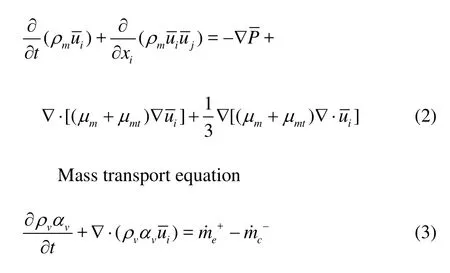
where?,P,μmandμmtrespectively represent the mean velocity, the mean pressure, the mixture fluid molecular viscosity and the turbulent viscosity,ρvandαvare the vapor phase density and volume fraction, respectively, the source terms?and?are derived from the cavitation model.
The mixture densityρmis defined as

wherefvis the mass fraction and the relation offvandvαis

1.2Turbulence model
In this research, the filter-based model[13]is used, which combines elements from both LES and RANS, and compares the characteristic length with the mesh size-spatial filter to reconstruct the turbulent viscosity

where the values of the turbulent kinetic energykand the turbulent kinetic dissipation rateεcome directly from the standardk-εmodel,Fis filter function, which is defined in terms of filter size Δ as
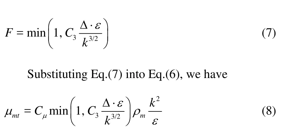
The proposed filter given in Eq.(7) recovers to the standardk-εmodel for a coarse filter size. In the far field zone the filter produces a hybrid RANSLES behavior by allowing the development of length scales comparable to grid resolution, and the turbulent viscosity becomes

where the value ofC3is chosen 1.0 for the present case.
In order to ensure that the numerically resolvable scale is compatible to the filtering process, the lower bound of the filter is set to be the grid size Δgrid, namely Δgrid=(ΔxΔyΔz)1/3.
1.3Cavitation model
The cavitation model, developed by Zwart et al., solves the following transport equation forαvin Eq.(3). The source termsm˙+andm˙-were derived
e
cfrom the bubble dynamics equation of the generalized Rayleigh-Plesset equation that account for mass transfer between the vapor and liquid phases in cavitation. They have the following forms:

The model involves four parameters and default values are used here. They are the bubble radiusRB= 10–6m, the nucleation site volume fractionrnuc=5× 10⁻⁴, the evaporation and condensation coefficientsFvap=50 andFcond=0.01.

Fig.1 Physical model of slanted axial-flow pump
In a slanted axial-flow pump, the internal flow is strongly unsteady turbulent flow, and the turbulent pressure fluctuations can lead to a local pressure decrease below the vapor pressure, which will easily lead to cavitation. Therefore, the influence of the turbulence on the cavitation process is considered. The approach to account for enhancement of cavitation due to turbulent pressure fluctuations is related to the turbulence kinetic energyk
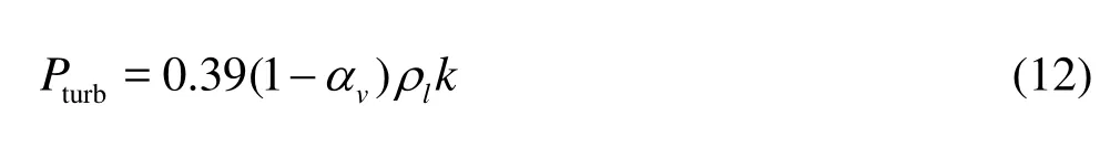
The vapor pressure is given as
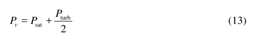
wherePsatis the saturation vapor pressure.

Fig.2 Grid for impeller and guider

Fig.3 Grid distribution for inlet flow channel and outlet flow channel

Table 1 Non-dimensional parameters
2. Physical model and computational method
2.1Physical model and mesh generation
The physical model of slanted axial-flow pump is shown in Fig.1(a), and Fig.1(b) shows the computational domain which consists of pump segment, inletflow channel and outlet flow channel. The pump segment consists of a 3-blade impeller and a 6-blade guider vane. The diameter of the impeller is 0.3 m, the gap of the blade tip clearance is 0.00015 m and the blade angle is –1.5o. The rotational speed of impeller is 1 450 rpm.

Table 2 Discretization error estimation
In order to effectively control the mesh distribution in the slanted axial-flow pump model, the whole hexahedral meshing strategy is adopted. The computational model is separated into four domains and each of them is connected by the interfaces which are set at the inlet and outlet of the impeller and guider vane. The grid is generated for each part by the software ANSYS ICEM CFD and the grid number and distribution are guaranteed consistently at the interface transition. Figures 2 and 3 show the mesh distribution in the pump segment, inlet flow channel and outlet flow channel. The O-type grid technology and local refinement method are adopted to control the near-wall mesh, which meets the requirements of corresponding turbulence model in the near-wall treatment. In order to obtain mesh-independent simulation results, the similar grid topology and distribution are kept for each part of the model. The discretization error in the performed CFD calculations is estimated and the results would be discussed in Subsection 2.4.
2.2Non-dimensional parameters
The calculated characteristics of the slanted axial-flow pump are presented by means of the nondimensional parameters, given in Table 1.
2.3Computational methodology
The three-dimensional, URANS equations were solved by using the CFD code ANSYS CFX. With automatic near-wall treatment, the turbulenct flow was simulated by the standardk-εmodel and the filterbased model, respectively. The second-order high resolution scheme and the second-order Backward Euler scheme were used separately for the advection term and transient term.
For the interface connection, the general grid interface was chosen for the reason that the grid on either side of the two connected surfaces permits nonmatching. The frozen rotor interface model was employed for the steady simulation and the results would be used as the initial flow field of the transient case. The transient rotor-stator interface model was utilized in the unsteady simulation which takes into account of all the transient flow characteristics and allows a smooth rotation between components.
For the boundary conditions, toward the hydraulic performance of slanted axial-flow pump under different operation conditions (noncavitating flow), the mass flow rate was given at the inlet and the average static pressure is imposed at the outlet, where the value relative to the atmospheric pressure was 0 Pa. However, in the cavitation simulation process, the constant mass flow rate was set at the outlet of model pump and the total pressure was specified at inlet, which relied on the cavitation condition. For transient case, the selected total time and time step size will be discussed in the next subsection.
2.4Numerical uncertainty analysis
A criterion of discretization error estimation named GCI method[14]which is based on the Richardson extrapolation technique[15]was utilized to improve grid resolution and systematically evaluate truncation error and accuracy. A representative grid sizehbased on the element volume and the grid refinement factorrwere defined as follows:

where ΔViis the volume of theith cell andNis the total number of cells used for the computations. Based on experience, the grid refinement factorris suggested greater than 1.3.
Three significantly different sets of grids were selected to make uncertainty analysis; the three sets of grids used were 410 521, 963 964, and 2 275 569 cells, respectively. The water-head coefficient and efficiency coefficient are selected as the values of the key variables. Table 2 gives the grid-refinement factorr, the solution valuesφ, the extrapolated solution valueφ21ext, the approximate relative errore21a, the extrapolated relative errorφ21extand the fine-grid convergence index GCI21fineon the basis of the water-head coefficientψand efficiency coefficientηat three flow rate coefficients:φ1=0.0678(0.767φBEP),φ2= 0.0883(φBEP) andφ1=0.108(1.223φBEP). Towards the fine grid number 2275569, at the three different flow ratess, the maximum of the extrapolated relative errorφ21extis 3.992% and 0.7368% for the water-head coefficientψand efficiency coefficientη, respectively. Moreover, the fine-grid convergence index GCI21finewas estimated to be below 5% in the region 0.0678<φ<0.108. Thus, the grid number 2 275 569 was chosen as the final computation number.

Table 3 Time step size and time duration (φBEP)
The discretization error analysis about the time step size and the time duration is also a mainly considerable problem in transient simulation. Five schemes are shown in Table 3, and the results are depicted in Fig.4. Considering the balance between the temporal accuracy and computing resource consumption, the scheme T2was chosen for the final computation due to its relative error of efficiency and water-head at the allowable range. At last, the time step size is set to 1.149×10⁻⁴s (about rotating 1oeach time step), and the total time of simulation is for impeller rotating 15 revolutions. The averaged results of the last five circles are exported for post-processing.
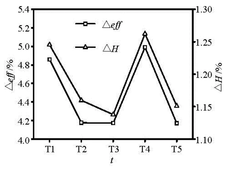
Fig.4 Analysis of the time resolution

Fig.5 Hydrodynamic performance curves for slanted axial-flow pump
3. Results and discussion
3.1Hydraulic performance characters
The comparison of hydrodynamic performance curves between numerical and experimental approaches in different operation conditions (non-cavitating flow) is shown in Fig.5. As can be seen from Fig.5, compared with the standardk-εmodel, numerical results with the filter-based model are in better agreement with the experimental results not only at the best efficiency point, but also under part-load condition. Moreover, the relative errors of both water-head coefficientψand efficiency coefficientηobtained by the filter-based model maintain smaller than 5%. Thus, the filter-based model was applied to simulate the unsteady cavitating flow within the slanted axial-flow pump.
3.2Cavitation performance
Net Positive Suction Head (NPSH) is usually used to describe the problem of cavitation in pumps, which could be expressed as
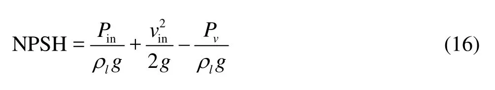
wherePinandvinare the static pressure and velocity in the fluid close to the impeller inlet, respectively.

Fig.6 Comparison of the relative errors of efficiency between simulation and experiment
Figure 6 demonstrates the comparison of cavitation performance for the slanted axial-flow pump between numerical simulation and experimental data at the best efficiency point. The comparison shows that the present numerical simulation results are in good agreement with the experimental data, especially the sudden decline tendency of the efficiency coefficientηcorresponding to the decrease of the NPSH. The critical NPSH, i.e., NPSHc, is defined as the NPSH value when the efficiency drops by 1%. In this study, their deviation between the obtained NPSHc values of 7.585 m in the experiment and 7.226 m in the calculation is about 4.73%. In addition, there are four different cavitation conditions where the internal flow fields would be investigated (marked in Fig.6): the non-cavitating conditiona(a′), the incipient cavitation conditionb(b′), the critical cavitation conditionc(c′) and the deep cavitation conditiond(d′).
3.3Discussion of internal flow
The flow field visualization tests have been carried out for four different conditions and the tip leakage cavitation patterns are showed in Fig.7. Figure 7(a) illustrates the noncavitating flow field, from which we can see that there are no visible signs of cavitation. Figure 7(b) shows that some small cavities are forming and shedding in the leading edge when the cavitation inception occurs. With decreasing the NPSH to the critical point, unstable cavitation is visible in this condition and large scale bubbly cavities shed but disappear instantly as shown in Fig.7(c). As Fig.7(d) shows, the deep cavitation condition leads to cavitation choking. As the cavity has significant thickness and there is significant cavitation reaching the trailing edge of the impeller blade, the passage flow area is greatly decreased and the hydrodynamic performance of the model pump is rapidly worsened.

Fig.7 Clearance and tip vortex cavitation pattern under different conditions
Computational results which illustrate the cavity size and shape along the impeller blade are shown in Fig.8. Compared with the cavitation patterns in Fig.7, the calculated cavity size and shape are similar to the experimental results in the respectively corresponding condition. Under noncavitating condition (as shown in Fig.8(a)), there are no cavitation occurring. Under the incipient cavitation condition, Fig.8(b) shows that some cavities appear at the leading edge and the tip clearance cavitation pattern also been observed. With the NPSH decreasing, under critical cavitation condition, the tip clearance becomes linked to the vortex ca-vitation and disappears rapidly. Especially under deep cavitation condition, the cavitation pattern becomes larger and isolated bubbles could also be observed in the flow field.
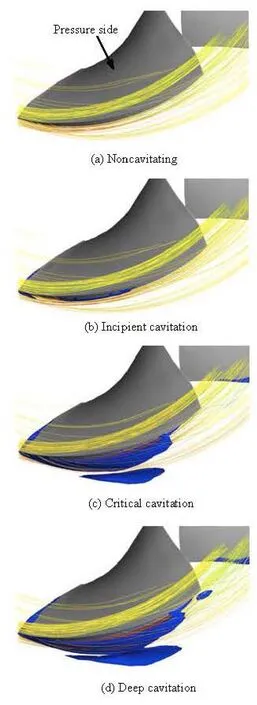
Fig.8 Calculated cavitation patterns at different NPSH (αv= 0.1)
In Figs.9 and 10, calculation results of the middle span from operating conditiona′ tod′ are presented in terms of local cavitation number (σN) and vapor volume. Figure 9 describes the degree of cavitation at different NPSHs and the dark blue color indicates a local saturated vapor flow. As the NPSH decreases,σNaround the blade foil is also declined. Meanwhile,σNin suction side is smaller than the value in the pressure side, which means the suction side is more likely to generate cavitation. Figure 10 plots the development of the cavity from noncaviting condition to the deep cavitation condition. Note that there is no evident cavitation in conditionsa′ andb′. At low NPSH condition,c′ andd′, the cavity generate clearly in the suction side, especially, cavitation reaches the trailing edge of the blade in deep cavitation condition and cavity choking appears easily.

Fig.9 Contours of local cavitation number (σN) at span 0.5
3.4BVF diagnosis
In this study, the Boundary Vorticity Flux (BVF)[16]has been applied to diagnose the internal cavitating flow inside the impeller passage of slanted axial-flow pump. The dynamics expression of BVF for incompressible fluid is defined as
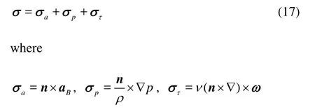

Fig.10 Contours of vapor volume fraction at span 0.5
The unknown parametersaσ,pσ,τσdenote the BVF which is created by the accelerated speed of surface boundaryaB, the pressure gradient ∇pand the boundary vorticityω, respectively. Considering the numerical simulation of axial-flow pump in this paper, the axial pressure gradientσpzis the only contributor to the BVF[17]. So chooseσpzas the flow diagnosis parameter

The BVF distribution and wall streamlines on blade suction surface for four different cavitation conditions are shown in Fig.11. In the noncavitating condition and incipient cavitating condition, the wall streamlines on the suction side surface are very smooth. As cavitation becomes deteriorating, the wall streamlines distribution on the blade suction side shows that a larger recirculation approaching to the trailing edge and forming the side-entrant jet. Under critical and deep cavitation condition, a prominent zone of positive BVF peak emerges near the trailing edge, which means there are vorticity concentrating.

Fig.11 BVF distribution on the suction side at different NPSHs
The cavitation patterns at different spans under critical and deep cavitation condtion are chosen to analyze the results in Fig.12. At different spans, the cavity shedding points(P1-P3,P4-P6) are affected by the side-entrant jet. The side-entrant jet, which is also influenced by the rotating blade, moves toward the cavity and thenthe cavity sheds fromthe blade suction surface into the impeller channel. Especially, under deep cavitation condition, the impeller channel are blocked by the large cavity (see Fig.8(d)). So the main flow are affected severely and the pump performance rapidly deteriorates.
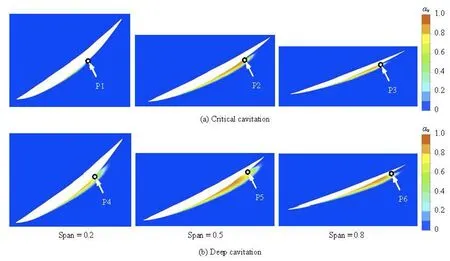
Fig.12 Cavity shedding for different spans
4. Conclusions
In the present paper, the hydraulic performance and cavitating flow behavior have been investigated by numerical simulation with slanted axial-flow pump model under different conditions. Based on the above results and discussions, the following conclusions can be drawn:
(1) Based on the URANS, the filter-based model has been applied to predict the hydraulic performance of pump model in noncavitating conditions and the results are proved in good agreement with the experimental results. On this basis, a numerical methodology with a mass transfer cavitation model is utilized to predict the cavitating flows in the pump model. And the cavitation performances are also well predicted.
(2) The cavitation internal flow analysis with the slanted axial-flow pump model indicates that the present computational methodology could capture the primary cavity structure, and the computational results coincide with the phenomenon of the observation experiment.
(3) The cavitating flow on the blade suction side has been diagnosed by the BVF. The results indicate that the cavitation performance drop is relevant to the shedding cavity, which is affected by the side-entrant jet.
[1] SENOCAK I., SHYY W. Interfacial dynamics-based modeling of turbulent cavitating flows, Part 1: Model development and steady-state computations[J]. International Journal for Numerical Methods in Fluids, 2004, 44(9): 975-995.
[2] LUCA D. A., MARIA V. S. Fluid dynamics of cavitation and cavitating turbopumps[M]. New York: Springer, 2008.
[3] KUMAR P., SAINI R. P. Study of cavitation in hydroturbines–A review[J]. Renewable and Sustainable Energy Reviews, 2010, 14(1): 374-383.
[4] ZHU Bing, CHEN Hong-xun. Cavitating suppression of low specific speed centrifugal pump with gap drainage blade[J]. Journal of Hydrodynamics, 2012, 24(5): 729-736.
[5] YANG Qiong-fang, WANG Yong-sheng and ZHANG Zhi-hong. Effects of non-uniform inflow on propeller cavitation hydrodynamics[J]. Chinese Journal of Hydrodynamics, 2011, 26(5): 538-550(in Chinese).
[6] KUNZ R. F., BOGER D. A. and STINEBRING D. R. et al. A preconditioned Navier-Stokes method for twophase flows with application to cavitation prediction[J]. Computers and Fluids, 2000, 29(8): 849-875.
[7] SINGHAL A. K., ATHAVALE M. M. and LI H. Mathematical basis and validation of the full cavitation model[J]. Journal of Fluids Engineering, 2002, 124(3): 617-624.
[8] ZWART P. J., GERBER A. G. and BELAMRI T. A. Two-phase flow model for predicting cavitation dynamics[C]. Fifth International Conference on Multiphase Flow. Yokohama, Japan, 2004.
[9] SCHNERR G. H., SAUER J. Physical and numerical modeling of unsteady cavitation dynamics[C]. Fourth International Conference on Multiphase Flow. New Orleans, USA, 2001.
[10] LIU S., NISHI M. and WU Y. et al. Cavitating turbulent flow simulation in a Francis turbine based on mixture model[J]. Journal of Fluids Engineering, 2009, 131(5): 051302.
[11] DING H., VISSER F. C. and JIANG Y. et al. Demonstration and validation of a 3D CFD simulation tool predicting pump performance and cavitation for industrial applications[J]. Journal of Fluids Engineering, 2011, 133(1): 011101.
[12] SAITO S., SHIBATA M. and FUKAE H. et al. Computational cavitation flows at inception and light stages on an axial-flow pump blade and in a cage-guided control Valve[J]. Journal of Thermal Science, 2007, 16(4): 337-345.
[13] JOHANSEN S. T., WU J. and SHYY W. Filter-based unsteady RANS computations[J]. International Journal of Heat and Fluid Flow, 2004, 25(1): 10-21.
[14] CELIK B. I., GHIA U. and ROACHE P. J. et al. Procedure for estimation and reporting of uncertainty due to discretization in CFD applications[J]. Journal of Fluids Engineering, 2008, 130(7): 078001.
[15] STEM F., WILSON R. V. and COLEMAN H. W. et al. Comprehensive approach to verification and validation of CFD simulations - Part 1: Methodology and procedures[J]. Journal of Fluids Engineering, 2001, 123(4): 793-802.
[16] WU J. Z., MA H. Y. and ZHOU M. D. Vorticity and vortex dynamics[M]. New York: Springer, 2006.
[17] ZHANG R., CHEN H. Numerical simulation and flow diagnosis of axial-flow pump at part-load condition[J]. International Journal of Turbo and Jet, 2012, 29(1): 1-7.
10.1016/S1001-6058(13)60411-4
* Project supported by the Key Research Projects of Shanghai Science and Technology Commission (Grant No.10100500200), the Science and Technology Plan of Zhejiang Province (Grant No. 2011C11068) and the Shanghai Program for Innovative Research Team in Universities.
Biography: ZHANG Rui (1984-), Male, Ph. D. Candidate
CHEN Hong-xun,
E-mail: chenhx@shu.edu.cn
猜你喜欢
杂志排行

水动力学研究与进展 B辑的其它文章
- Hydrodynamic effects on contaminants release due to rususpension and diffusion from sediments*
- The influence of the flow rate on periodic flow unsteadiness behaviors in a sewage centrifugal pump*
- Practical evaluation of the drag of a ship for design and optimization*
- Inverse problem of bottom slope design for aerator devices*
- Assessment of ship manoeuvrability by using a coupling between a nonlinear transient manoeuvring model and mathematical programming techniques*
- Generation and evolution characteristics of the mushroom-like vortex generated by a submerged round laminar jet*