WELL TESTING ANALYSIS FOR HORIZONTAL WELL WITH CONSIDERATION OF THRESHOLD PRESSURE GRADIENT IN TIGHT GAS RESERVOIRS*
2012-08-22GUOJingjing
GUO Jing-jing
State Key Laboratory of Oil and Gas Reservoir Geology and Exploitation, Southwest Petroleum University, Chengdu 610500, China, E-mail: gjjswpu@126.com
ZHANG Su
Central Sichuan Mining District, PetroChina Southwest Oil and Gas Field Company, Suining 629000, China
ZHANG Lie-hui
State Key Laboratory of Oil and Gas Reservoir Geology and Exploitation, Southwest Petroleum University, Chengdu 610500, China
QING Hairuo
Department of Geology, University of Regina, Regina, SK S4S 0A2, Canada
LIU Qi-guo
State Key Laboratory of Oil and Gas Reservoir Geology and Exploitation, Southwest Petroleum University, Chengdu 610500, China
(Received January 4, 2012, Revised April 18, 2012)
WELL TESTING ANALYSIS FOR HORIZONTAL WELL WITH CONSIDERATION OF THRESHOLD PRESSURE GRADIENT IN TIGHT GAS RESERVOIRS*
GUO Jing-jing
State Key Laboratory of Oil and Gas Reservoir Geology and Exploitation, Southwest Petroleum University, Chengdu 610500, China, E-mail: gjjswpu@126.com
ZHANG Su
Central Sichuan Mining District, PetroChina Southwest Oil and Gas Field Company, Suining 629000, China
ZHANG Lie-hui
State Key Laboratory of Oil and Gas Reservoir Geology and Exploitation, Southwest Petroleum University, Chengdu 610500, China
QING Hairuo
Department of Geology, University of Regina, Regina, SK S4S 0A2, Canada
LIU Qi-guo
State Key Laboratory of Oil and Gas Reservoir Geology and Exploitation, Southwest Petroleum University, Chengdu 610500, China
(Received January 4, 2012, Revised April 18, 2012)
A fundamental solution for homogeneous reservoir in infinite space is derived by using the point source function with the consideration of the threshold pressure gradient. The fundamental solution of the continuous point source function is then derived based on the Green function. Various boundary conditions of the reservoirs are considered for this case and the corresponding solutions are obtained through the mirror image reflection and the principle of superimposition. The line source solution is obtained by integration. Subsequently, the horizontal-well bottom hole pressure response function for a non-linear gas flow in the homogeneous gas reservoir is obtained, and the response curve of the dimensionless bottom hole pressure and the derivative for a horizontal well in the homogeneous gas reservoir are obtained. In the end, the sensitivities of the relevant parameters are analyzed. The well test model presented in this paper can be used as the basis of the horizontal well test analysis for tight gas reservoirs.
horizontal well, non-linear gas flow, threshold pressure gradient, tight gas reservoir
Introduction
In the early 1987, the concept of the threshold pressure gradient was introduced into the petroleum industry. Subsequent studies have confirmed the exi-stence of the threshold pressure gradient in tight gas reservoirs. Due to large pore throats in conventional gas reservoirs, the threshold pressure gradient has little effect on the well performance and can be neglected. However, with significantly smaller pore throats in tight gas reservoirs, the effect of the threshold pressure gradient might be significant and should be considered for the prediction of the well performance.
The horizontal well test analysis models were first developed during the 1980s. Clonts and Ramey[1]derived one of the earliest analytical solutions for the horizontal well test analysis, based on the line source approximation for a vertical partially penetrated fracture well, with the assumption that a horizontal wellcould be viewed as a well producing from a line source in an infinite-acting reservoir. These models have three major limitations: (1) the wellbore pressure is calculated at a finite radius outside the source and it is therefore impossible to obtain the wellbore pressure within the source, (2) it is difficult to conduct a realistic productivity comparison between a horizontal well and a vertical fractured well, (3) the line source approximation may not be adequate for reservoirs with thin pay zones.
During the 1990s, some new models were developed to eliminate the limitations of the earlier horizontal well models. However, the fundamental assumptions and the methodology employed in the development of these new set of solutions remain virtually the same as those of the earlier models. Ozkan[2]presented one of the most compelling arguments that the horizontal wells require realistic models and concepts which are robust enough to meet the increasingly challenging task of the accurate evaluation of the horizontal well performance. Ozkan’s work presented a critique of the conventional and contemporary horizontalwell-test analysis procedures that they will not be adeof conditions. Ogunsanya et al.[3,4]developed a new quate and the margin of error is associated with a set type curve solution for a hydraulically fractured horizontal well producing from a solid bar source in an infinite-acting reservoir. A dimensionless rate function was introduced to convert the pressure response of a horizontal well into the equivalent response of a vertical fractured well.
In the 20th century, Ozkan[5,6]presented a discussion of the fractured horizontal-well performance in conventional and tight reservoirs. Based on Ozkan’s studies, Brown et al.[7]presented an analytical trilinear flow solution to simulate the pressure transient and production behavior of fractured horizontal wells in tight reservoirs.
Some models were also proposed to study the pressure dynamics for vertical wells with consideradual porosity reservoirs[8-12]. However, to the best of tion of the threshold pressure gradient in single and our knowledge, little progress has been made on horizontal well test models with consideration of the threshold pressure gradient in tight gas reservoirs. Therefore, this paper proposes a transient mathematical model for horizontal wells with consideration of the threshold pressure gradient which is more suitable for general tight gas reservoirs. Subsequently, the horizontal well bottom hole pressure response function for a non-linear gas flow in a homogeneous gas reservoir is constructed. The response curve of the horizontal well in the form of the dimensionless bottom hole pressure and its derivative for the homogeneous gas reservoir are obtained. In the end, the sensitivities of related parameters are analyzed.

Fig.1 Schematic diagram of infinite space unit
1. Point source function in an infinite space
As shown in Fig.1, let Ω be an arbitrary subdomain within the boundary B, and n be the outward unit normal to dΓ, a surface element of the boundary B of the study area. M is a volume element dV at any point within the boundary B. According to the law of conservation of mass, the overall fluid quantity in the hierarchy of control should be equal to the mass difference between the inflow and the outflow.

where D is the space-time domain, φ is the porosity, ν is the flow velocity, ρ is the density and t is the time varia- ble.
We restrict our attention to Newtonian fluids and isothermal conditions, and the reservoir is considered homogeneous in all rock properties and isotropic with respect to permeability. Ignoring gravity and capillary pressure, the equation governing the flow with consideration of the threshold pressure gradient can be derived from the equation of state, the motion equation and the continuity equation, which is expressed in terms of the pseudo pressure.

where ψ is the pseudo pressure for the real gas,, k is the permeability, μ is the viscosity for the gas, Z is the gas compressibility coefficient,ic is the total compressibility of the porous medium, η is the diffusivity of the porous solid, η=k/(φμct), λψBis the (pseudo) threshold pressure gradient , λψB=2piλBL/μZ, λBis the threshold pressure gradient,ip is the reference pressure, L is the reference length.
Let iD=i/L, i=x,y,z, tD=ηt/L2, Δψ= ψi-ψ. Then we obtain the dimensionless form of Eq.(2) as follows

whereDt is the dimensionless time.
The Laplace transformation of Eq.(3) yields

where s is the Laplace transform variable.
For a point source located at the origin in an isotropic system, we can write Eq.(4) with the consideration of the threshold pressure gradient in the spherical coordinates as

and

whereDρ is the dimensionless spherical radial distance.
The boundary condition at the surface of a vanishingly small sphere corresponding to the instantaneous withdrawal of an amount of fluid1q~ at =0t can be expressed by

where ε is the micro variable,1q~ is the production rate from a point source, T is the temperature,scp andscT are the pressure and the temperature under the standard condition.
The Laplace transform of Eq.(6) gives

For simplicity, assume that the strength of the source is unity, then Eq.(7) can be written as


By using the pre-solution[13]method, the general solution of Eq.(9) is

That is the fundamental solution of the instantaneous point source function in the Laplace space. It is worth pointing out that the first term in Eq.(10) is directly related to a point source strength and the second term is related to the threshold pressure gradient. WhenBψλ is equal to zero, Eq.(10) is the instantaneous fundamental solution without consideration of the threshold pressure gradient.
Considering the strength of the source, the instantaneous fundamental solution is

When a point source function in the center withdraws a continuous liquid from 0 to t, the fundamental solution of a continuous point source in the physical space is given by

where

Unless explicitly specified, we will assume that the source distribution in time and over the integration path in Eq.(12) is uniform. Thus we have


Fig. 2 Schematic diagram of a horizontal well in infinite formation
2. Mathematical models of horizontal well
The physical model of a horizontal well is schematically shown in Fig.2. The key assumptions are:
(1) The reservoir is horizontal, homogeneous, anisotropic with the constant horizontal permeability khand the constant vertical permeability kv, the thickness h, and the porosity φ. The reservoir can be infinite or finite in the lateral extension. The reservoir is bounded with closed top and bottom boundaries.
取平均值ΔL为17.5 dB/m,ΔL0对于本设备取120 dB,计算出消声器长度为L=1 010 mm.
(2) The reservoir pressure is constant in the initial condition. Gravity effect and capillary pressure are considered to be negligible.
(3) The well is assumed to be parallel to the top and the bottom sealing boundaries, to be located at any locationwz, from the bottom, and its length is 2L. The well radius iswr.
(4) Single-phase fluid and constant rate production,scq.
According to the fundamental solution to a continuous point source in an infinite space, Eq.(13), the fundamental solution under impermeable upper and lower boundary conditions can be obtained by using the mirror images and the principle of superposition, which is given by

where


Equation (14) is the continuous point source solution for the laterally infinite system. Assume that the gas reservoir is a close system with a cylindrical surface boundary located at RD=ReD. In the case where the boundary conditions at zD=0 and 1 and at RD=ReDare all impermeable, a solution in the following form can be constructed

In Eq.(15), P is a solution that satisfies the inner boundary condition and the impermeable boundary conditions at zD=0 and 1. G is also a solution that satisfies the boundary condition at zD=0 and 1, and P+G satisfies the boundary conditions at RD= ReDand the inner boundary condition. Then we can choose the solution Eq.(14) as P. Since Eq.(14) satisfies the inner boundary condition, the contribution of G to the inner boundary condition vanishes as RD→0. We can get the expression of G as follows by using the Muskat’s method

where

Thus, the continuous point source solution for the laterally closed system can be written as


Equations (14) and (17) are the continuous point source solutions for laterally infinite and laterally closed systems with impermeable top and bottom boundaries, respectively.
The solution for a horizontal line-source well of length 2L can be obtained from the integration of the right side of Eqs.(14) and (17) from (xw-L) to (xw+L) with respect to xw. The pressure distribution for the horizontal well in a laterally infinite reservoir with boundaries of two impermeable planes at z=0 and z=h can be written as

where

The pressure distribution for a horizontal well in a laterally bounded reservoir with boundaries of two impermeable planes at =0z and =zh, can be written as

where

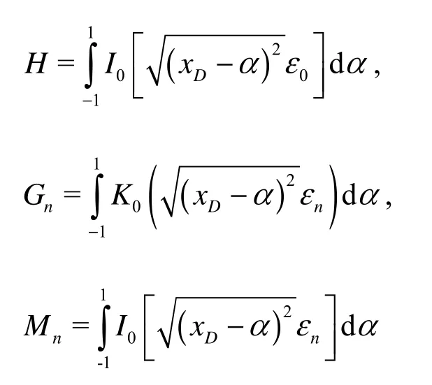
The preceding solutions give the horizontal-well pressure response functions for various boundary conditions. However, the wellbore storage and skin effects have not yet been taken into account. By using the Duhamel principle, the dimensionless well bottom pressure of the horizontal wells with the wellbore storageDC and the skin effects S and in the Laplace domain is obtained as

where

3. Analysis of type curve features
According to the solution of the mathematical model for a horizontal well in tight gas reservoirs, the pressure and the derivative type curves that reflect the horizontal well pressure behavior in laterally infinite gas reservoirs are obtained by using the Stehfest numerical reversion algorithm[14,15]. The results are shown in Figs.3-4.
Figure 3 is a dimensionless pressure and pressure-derivative log-log type curve for a horizontal well with differentDλ in an infinite gas reservoir with a sealing top and bottom boundaries. When the threshold pressure gradient is considered, there is an obviously pressure behavior change in the fourth flow regime. The fourth flow regime can be further divided into two phases, the late horizontal pseudo-radial flow and the upwarping flow. In other word, the effect of the threshold pressure gradient on the pressure behavior mainly exists in the med-late periods. It leads to a gradual growth of the pressure drawdown and an upwarping of the pressure and derivative curves. The greater the threshold pressure gradient is, the steeper the upwarping feature will be. The upwarping seg-ment of the curve usually appears after the late horizontal pseudo-radial time period. However, whenDλ is too large, the previous flow regime can become deceitful. The effect of the threshold pressure gradient on the relationship between the derivative and the time shows mainly in this stage. With the growth ofDλ, the fourth flow regime shows up earlier, butDλ has no obviously effect on the other flow regimes.

Fig.3 The effect of threshold pressure gradient on horizontal gas well pressure behavior (Pe=30MPa , TR=80oC , rw=0.1m , γg=0.65, β=5, CDe2s=300, LD=10, hD=300,zwD=0.5)

Fig.4 The effect of dimensionless length on horizontal gas well pressure behavior (Pe=30MPa , TR=80oC , rw= 0.1m, γg=0.65, β=5, CDe2s=300, λD=0.005, hD=300,zwD=0.5)
Figure 4 is a dimensionless pressure and pressure-derivative log-log type curve of one horizontal well with different dimensionless lengthDL in an infinite gas reservoir with a sealing top and bottom boundaries. Figure 4 shows that the effect of the threshold pressure gradient on the curve shows mainly in the upwarping flow regime after the late horizontal radial flow time period. WhenDλ is given, the smaller the value ofDL is, the earlier the upwarping of the curve appears, and vice versa. The reason lies in the condition that the other parameters are invariant. The smaller the value ofDL is, the shorter the horizontal length is and the smaller its the drainage area will be. The resistance to the flow becomes relatively greater, and the corresponding drawdown pressure will be greater. Because the permeability and the threshold pressure gradient are given, the upwarping of the pressure and derivative curves shows up earlier.
Similar to the previous process, based on the solution of the mathematical percolation model for a horizontal well in a closed external boundary gas reservoir with a sealing top and bottom boundaries, the pressure and derivative type curves for a horizontal well are obtained and plotted in Figs.5-6.

Fig.5 The effect of threshold pressure gradient on horizontal gas well pressure behavior (Pe=30MPa , TR=80oC , rw=0.1m , γg=0.65, β=5, CDe2s=300, LD=10, hD=300,reD=10)

Fig.6 The effect of dimensionless length on horizontal gas well pressure behavior (Pe=30MPa , TR=80oC , rw= 0.1m, γg=0.65, β=5, re=3000, CDe2s=300, hD=300,λD=0.01)
Figure 5 shows the dimensionless pressure and its derivative type curves of a single horizontal gas well in a laterally closed gas reservoir with a sealing top and bottom boundaries. From the derivative curve, it can be seen that the flow behavior is identical to that of the infinite situation before the pressure wave propagates to the circular outer boundary. After the pressure wave reaches the circular closed outer boundary, it is shown that the pseudo-stable flow behavior is controlled by the closed outer boundary. The greater the threshold pressure gradient is, the earlier the upwarping of the derivative curve will be. The derivative is a straight line with a certain slope related to the value ofDλ and less than 1. In addition, the pseudostable flow behavior appears earlier. When the value ofDλ exceeds a certain value, the previous flowregime might be deceitful. The above features of the derivative curve are caused by the combination of the effects of the threshold pressure gradient and the closed outer boundary.
Figure 6 shows the dimensionless pressure and its derivative log-log type curves for a single horizontal gas well with differentDL in a laterally closed gas reservoir with a sealing top and bottom boundaries. With or without considering the effect of the threshold pressure gradient, the appearance of the pseudo-stable radial flow is not related to the length of the horizontal wells. However, due to the existence ofDλ, the upwarping feature caused by the effect of the closed boundary comes relatively earlier. With the decrease ofDL, the late horizontal pseudo-stable flow shows up earlier. The reverse is true whenDL increases.
4. Model validation
In this section, a horizontal production well located in a tight gas reservoir is considered. The relevant parameters of the well are as follows. The reservoir thickness is 12.6 m, the well length of the horizontal section is 735.23 m, the well radiuswr is 0.1 m, the average porosity is 0.1, and the reservoir temperature and the initial pressure are 405 K and 42.11 MPa, respectively. The well has been in production for 34.15 h at a rate of 36.59×10⁴ m3/d before the pressure buildup test and the PBU well test lasts 238.59 h. The fluid viscosity is 0.03362 cp. The Z-factor is 0.9114, and the total compressibility is 0.01516 MPa-1.

Fig.7 Log-log fitting curves of actual well test data
The log-log fitting curves are shown in Fig.7. The parameter λ can be calculated by the fitting resultsDλ. The obvious upwarping tendency caused by the threshold pressure gradient can be observed from the fitting curves in a late time.
The fitting results are as follows: the permeability is 6.746 mD, and the wellbore storage factor is 0.1429 m3/MPa, and the calculated threshold pressure gradient is 0.00034 MPa/m.
5. Conclusions
(1) The horizontal gas well models with consideration of the threshold pressure gradient is established in this paper and they can be used as the theoretical basis of the horizontal well test analysis for tight gas reservoirs.
(2) The bottom hole pressure response function for the horizontal gas well with consideration of the threshold pressure gradient in various boundary conditions is derived by using the fundamental solution of the point source function in the Laplace domain.
(3) The effect of the threshold pressure gradient on the pressure behavior for horizontal gas wells mainly shows in the med-late time periods. The upwarping feature of the type curves appears earlier with the increase ofDλ value, and vice versa. The threshold pressure gradient has a negligible effect on the previous flow regimes.
(4) For an infinite gas reservoir, with fixedDλ, the smaller the value ofDL is, the earlier the upwarping feature of the type curves appears, and vice versa. For a laterally closed gas reservoir, the appearance of the pseudo-stable radial flow is independent of the well length of the horizontal section. However, due to the existence ofDλ, the upwarping feature of the type curves is caused by the closed boundary conditions.
Acknowledgement
This worked was supported by the Research Foundation of the State Key Laboratory of Oil and Gas Reservoir Geology and Exploitation, Southwest Petroleum University (Grant No. PLN-ZL201201).
[1] CLONTS M. D., RAMEY H. J. Pressure transient analysis for wells with horizontal drainholes[C]. SPE 15116. Oakland, California, USA, 1986, 215-230.
[2] OZKAN E. Analysis of horizontal-well responses: Contemporary vs. conventional[J]. SPE Reservoir Evaluation and Engineering, 2001, 4(4): 260-269.
[3] OGUNSANYA B. O. A physically consistent solution for describing the transient response of hydraulically fractured and horizontal wells[D]. Ph. D. Thesis, Lubbock, Texas, USA: Texas Tech University, 2005.
[4] OGUNSANYA B. O., OETAMA T. P. and LEA J. F. et al. A coupled model for analyzing transient pressure behavior of horizontal drainholes[C]. SPE 94331. Oklahoma City, Oklahoma, USA, 2005, 1-14.
[5] OZKAN E. Comparison of fractured horizontal-well performance in conventional and unconventional reservoirs[C]. SPE 121290. San Jose, California, USA, 2009, 1-16.
[6] OZKAN E., BROWN M. and RAGHAVAN R. et al. Comparison of fractured-horizontal-well performance in tight sand and shale reservoirs[J]. SPE Reservoir Evaluation and Engineering, 2011, 14(2): 248-259.
[7] BROWN M., OZKAN E. and RAGHAVAN R. et al. Practical solutions for pressure transient responses of fractured horizontal wells in unconventional reservoirs[J]. SPE Reservoir Evaluation and Engineering, 2011, 14(6): 663-676.
[8] LIANG Bin, LI Min and ZENG Fanhua et al. Study on the analytical solution of mathematical model for the tight gas reservoir about start-up gradient[J]. Fault-Block Oil and Gas Field, 2004, 11(6): 31-34(in Chinese).
[9] LIU Qi-guo, YANG Xu-ming and WEI Hong-mei et al. Study of well-test model of low permeability’s dualpore media with flowing boundary in oil and gas[J]. Journal of Southwest Petroleum Institute, 2004, 26(5): 30-33(in Chinese).
[10] ZHANG Yun, WANG Zi-sheng and YAO Jun et al. Study and application of pressure transient of naturally fractured reservoirs with stree-sensitive and start pressure grade[J]. Journal of Hydrodynamics, Ser. A, 2007, 22(3): 332-337(in Chinese).
[11] FENG Guo-qing, LIU Qi-guo and SHI Guang-zhi et al. An unsteady seepage flow model considering kickoff pressure gradient for low-permeability gas reservoirs[J]. Petroleum Exploration and Development, 2008, 35(4): 457-461(in Chinese).
[12] CHENG Lin-song, REN Sheng-li and LIAN Pei-qing. Well test analysis on low velocity and non-Darcy flow in dual-porosity reservoir with dynamic boundary[J]. Chinese Journal of Computational Mechanics, 2011, 28(6): 879-883(in Chinese).
[13] ZHANG Xue-yuan. The resolvent method of solving second order variable coefficient linear non-homogeneous differential equation[J]. Journal of Shanghai Second Polytechnic University, 2004, (1): 1-7(in Chinese).
[14] ZHANG Llie-hui, GUO Jing-jing and LIU Qi-guo. A new well test model for a two-zone linear composite reservoir with varied thicknesses[J]. Journal of Hydrodynamics, 2010, 22(6): 804-809.
[15] GUO J., ZHANG L. and WANG H. et al. Pressure transient analysis for multi-stage fractured horizontal wells in shale gas reservoirs[J]. Transport in Porous Media, 2012, 93(3): 635-653.
10.1016/S1001-6058(11)60278-3
* Project supported by the National Science Fund for Distinguished Young Scholars of China (Grant No. 51125019), the National Key Basic Research and Development Program of China (973 Program, Grant No. 2011CB201005).
Biograophy: GUO Jing-jing (1986-), Female, Ph. D. Candidate
ZHANG Lie-hui,
E-mail: zhangliehui@vip.163.com
猜你喜欢
杂志排行

水动力学研究与进展 B辑的其它文章
- EXPERIMENTAL STUDY OF CONDENSATION HEAT TRANSFER CHARACTERISTICS OF HORIZONTAL TUBE BUNDLES IN VACUUM STATES*
- THE NATURAL CONVECTION OF AQUIFERS WITH CONSTANT HEAT SOURCES AND ITS INFLUENCE ON TEMPERATURE FIELDS*
- EFFECT OF ESCAPE DEVICE FOR SUBMERGED FLOATING TUNNEL (SFT) ON HYDRODYNAMIC LOADS APPLIED TO SFT*
- EXPERIMENTAL STUDY OF AIRFLOW INDUCED BY PUMPING TESTS IN UNCONFINED AQUIFER WITH LOW-PERMEABILITY CAP*
- SIMULATION OF HYDRAULIC TRANSIENTS IN HYDROPOWER SYSTEMS USING THE 1-D-3-D COUPLING APPROACH*
- TOTAL PHOSPHORUS RELEASE FROM BOTTOM SEDIMENTS IN FLOWING WATER*