SIMULATION OF HYDRAULIC TRANSIENTS IN HYDROPOWER SYSTEMS USING THE 1-D-3-D COUPLING APPROACH*

ZHANG Xiao-xi, CHENG Yong-guang

State Key Laboratory of Water Resources and Hydropower Engineering Science, Wuhan University, Wuhan 430072, China, E-mail: zhangxiaoxi@whu.edu.cn

(Received May 28, 2012, Revised June 19, 2012)

SIMULATION OF HYDRAULIC TRANSIENTS IN HYDROPOWER SYSTEMS USING THE 1-D-3-D COUPLING APPROACH*

ZHANG Xiao-xi, CHENG Yong-guang

State Key Laboratory of Water Resources and Hydropower Engineering Science, Wuhan University, Wuhan 430072, China, E-mail: zhangxiaoxi@whu.edu.cn

(Received May 28, 2012, Revised June 19, 2012)

Although the hydraulic transients in pipe systems are usually simulated by using a one-dimensional (1-D) approach, local three-dimensional (3-D) simulations are necessary because of obvious 3-D flow features in some local regions of the hydropower systems. This paper combines the 1-D method with a 3-D fluid flow model to simulate the Multi-Dimensional (MD) hydraulic transients in hydropower systems and proposes two methods for modeling the compressible water with the correct wave speed, and two strategies for efficiently coupling the 1-D and 3-D computational domains. The methods are validated by simulating the water hammer waves and the oscillations of the water level in a surge tank, and comparing the results with the 1-D solution data. An MD study is conducted for the transient flows in a realistic water conveying system that consists of a draft tube, a tailrace surge tank and a tailrace tunnel. It is shown that the 1-D-3-D coupling approach is an efficient and promising way to simulate the hydraulic transients in the hydropower systems in which the interactions between 1-D hydraulic fluctuations of the pipeline systems and the local 3-D flow patterns should be considered.

hydropower station, hydraulic transients, compressible water model, coupling of 1-D and 3-D methods

Introduction

The variations of the operating conditions in a hydropower system will lead to transients due to the fluctuations of the parameters in the hydraulic, mechanical and electrical systems, which are closely related with the safety and the operating stability[1,2]of the whole system. Among these processes, the hydraulic transients always produce enormous hydraulic waves, which may result in catastrophes in extreme cases. Therefore, it is important to carefully analyze the hydraulic transients in any hydropower station during the design stage[3].

Due to the hydraulic transients, the flow patterns in some local regions of a water conveying system present obvious three-dimensional (3-D) features. For example, the water surface in a long corridor-shaped surge tank oscillates rapidly in vertical and longitudi-nal directions. Moreover, some harmful air-entraining vertical vortices may be generated around the orifice when the water level is low. As the 3-D flow patterns in these local regions might interact strongly with the flow of the whole water conveying system, the traditional one-dimensional (1-D) methods are not applicable in studying this problem.

Since the 1970s, several Multi-Dimensional (MD) methods based on the Method Of Characteristics (MOC)[1]were proposed and applied successfully in MD transient flow simulations. However, these methods did not find wide applications because of limitations such as the poor numerical stability, the complicated solution schemes and the fixed grids[4]. With the development of mathematical models and numerical methods for fluid flows, the Computational Fluid Dynamics (CFD) is widely used to simulate some hydraulic transients. For instance, Kolsek et al.[5]predicted the characteristics of a bulb turbine in the case of a sudden load rejection, and the simulated results agree well with the experimental data, which validated the CFD method in simulating the transients in the hydraulic machinery. Cheng et al.[6]applied the CFD with the Volume Of Fluid (VOF) model to simu-late the transient flow in a Ceiling-Sloping Tailrace Tunnel (CSTT) during the load rejection process, and the results show that the VOF-CFD method performs better than the existing 1-D method in both physical interpretation and numerical accuracy. Cheng and Suo[4]established a Lattice Boltzmann Method (LBM) of the CFD for the 2-D water hammer simulation in a concrete spiral case, and it is shown that the model might be used for the MD hydraulic transients.

However, practically the CFD method is not mature enough to be applied for MD simulations of hydraulic transients in hydropower systems for two reasons. On one hand, the water is always treated as an incompressible fluid for general CFD models. This treatment is reasonable in most cases, but not suitable for simulating the “water hammer” phenomenon, caused by the compressibility of the water and in which the pressure wave propagates with a finite speed and is reflected by the boundaries, for hydraulic transients in hydropower systems. With the incompressible assumption, some unphysical errors will arise, such as the overpressure for a sudden closing of the valve would be far greater than that in the actual case. On the other hand, because the water conveying system is always very long, it is neither necessary nor feasible to simulate the whole system with a 3-D model. If only some local 3-D regions are of interest, the varying boundary conditions in transients would be very complex. Therefore, the compressible water model and the 1-D-3-D coupling method are the issues to be addressed. For the first issue, Yan et al.[7]proposed a method of modeling the 3-D compressible water in the commercial CFD software CFX for studying the influence of the water compressibility on the pressure fluctuations induced by the rotor-stator interaction in pump-turbines in a steady condition. Nevertheless, their studies did not consider the field of hydraulic transients. For the second issue. Lin et al.[8]developed a model of coupling 1-D and 3-D CFD equations for simulating MD gas flows in the human lung, Han et al.[9]simulated a huge channel network system by coupling 1-D and 2-D channel flow models. In the field of hydropower engineering, Ruprecht et al.[10,11]proposed a method for coupling 1-D MOC and 3-D CFD when studying the pressure fluctuations in a draft tube, Cherny et al.[12]used this method to simulate the runaway process of a Francis turbine. However, this method involves some limitations, which will be discussed later in this paper.

This paper will model the compressibility of the water and couple the 1-D and 3-D computational domains, with the existing CFD software, to simulate the MD hydraulic transients in hydropower systems efficiently and accurately.

1. Methods for modeling compressible water

If the pressure increases, the water will be compressed, resulting in an increase in density. Therefore, besides the continuity and momentum equations, there must be a state equation to relate the density with the pressure in the CFD equations for the compressible water. Here, we use the commercial CFD software Fluent and provide two methods for dealing with the state equation of water.

1.1 Defining a Density Function (DDF)

The state equation for water is given as

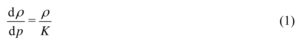
where ρ is the density, p is the relative pressure, and K is the bulk modulus of elasticity. From Eq.(1), we obtain

where0p and0ρ are the relative pressure and density in the initial state. In addition, under the standard conditions of an ambient temperature at 20oC and an absolute pressure of one atmosphere, the value of0p is 0 Pa and0ρ is 998.2 kg/m3.

The general acoustic wave speed a of water in pipe can be expressed as[13]

where D is the pipe radius, e is the pipe-wall thickness, E is the Young’s modulus of elasticity of the pipe-wall, c is a coefficient related to the anchored condition and the wall thickness of the pipe.

In an infinite water environment with a small disturbance, Eq.(3) can be simplified to

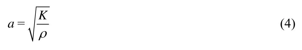
For water, the change in a is so small that it could be regarded as a known constant, then, Eq.(4) can be written as

where0a is the acoustic wave speed in the initial state. Substituting Eq.(5) into Eq.(2), we obtain

If the effect of the pipe-wall elasticity is taken into account,0a can be calculated from Eq.(3).

The software Fluent provides the function of a user defined density, which enables the user to customize the density as a function of other flow variables using the User Defined Function (UDF) procedures. Here we take the water state equation (Eq.(6)) as the density function and solve it explicitly at every step after the pressure p is obtained.

This method has a definite physical meaning because it is based on the state equation of the water. However, it is an explicit scheme, which means that the time step must be small enough to maintain a good accuracy.

1.2 Modifying the Ideal Gas Law (MIGL)

The ideal gas law for compressible gas in Fluent provides a relationship between the density and the pressure. Here, the compressibility of water can be modeled by modifying the parameters. The ideal gas law may be written as[14]

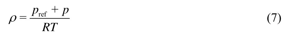
where prefis the reference pressure, p is the relative pressure, T is the temperature on the Kelvin scale, and R=R0/M, where R0=8314.5 J/K-kmol is the universal gas constant and M is the molecular weight.

The acoustic speed for the ideal gas is given by

where γ=cp/cvis the ratio of specific heats, with cpas the constant pressure specific heat and cvthe constant volume specific heat. Assuming that cv= cp-R, one can express γ as

Also it is assumed that a is a known constant in water. From Eq.(8), T can be written as

Substituting Eq.(10) into Eq.(7), we obtain

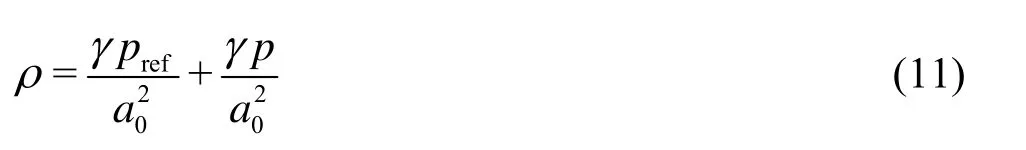
Yan et al.[7]suggested that the state equation of water could be expressed as

So we can solve therefp and γ by comparing Eq.(12) and Eq.(11), and obtain:

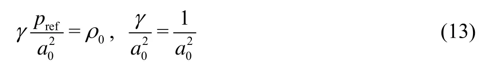
Then

If γ=1, it becomes evident that the cpmust be much larger than R according to Eq.(9). We let cp=109Jkg-1K-1.

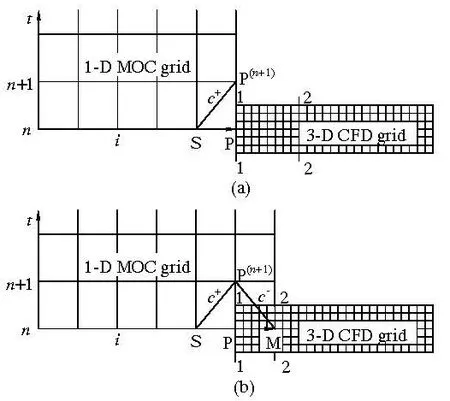
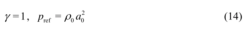
Fig.1 Schematic diagram of 1-D and 3-D coupling

Providing we modify the values of T, prefand cp, the ideal gas law (Eq.(7)) can be approximately taken as the state equation of water (Eq.(12)). Therefore, the compressible water can be simulated through this model. Note that, T, prefand cphere are only used as coefficients of an equation and do not have any physical meaning. More importantly, because the solution is about water, all other parameters, such as density, viscosity and molecular weight, must be based on the properties of water.

Th is method is rel atively s imple and o nl y requiresthemodificationofseveralparametersinFluent.However, it is unreliable in terms of its physical meaning. Meanwhile this method is also in an explicit scheme. Additionally, it needs to be solved with the energy equation, which would consume more computational resources than the DDF.

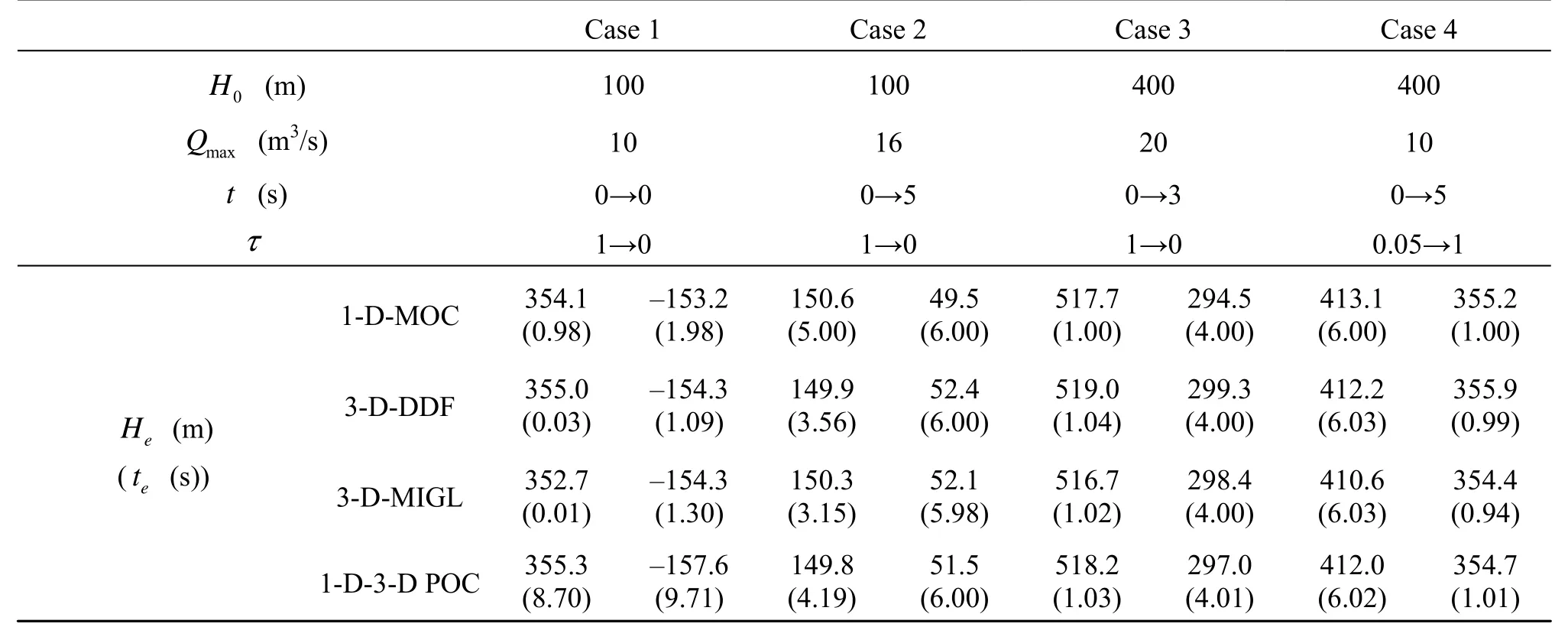
Table 1 Computational conditions and results of water hammer simulations

2. 1-D-3-D coupling methods

2.1 The basic idea and the existing method for 1-D-3-D coupling

The basic idea of the 1-D-3-D coupling is to divide one complex computational domain into two parts according to the flow patterns. The strip parts, such as a pipeline, where the flow variables change almost only along the central streamline, can be simplified to a 1-D line and analyzed by the MOC. As for the part where the streamlines change rapidly in a short distance, such as in a surge tank and the hydraulic turbine, the 3-D CFD method is used. The most important operation is to develop a method of data exchange at the 1-D-3-D coupling boundary.

Consider a simple system, consisting of a 1-D MOC grid upstream and a 3-D CFD grid downstream, as shown in Fig.1(a). The node P in the MOC grid or the Section 1-1 in CFD grid is the interface between the two parts where the node P is located in the section 1-1. Note that the data formats stored in them are different, that is, the data are of the integral form in the node P but the discrete form in the Section 1-1.

Initially, assume that the flow variables at the time step n are known at all grid nodes, including the 1-D and 3-D parts. Correspondingly, for the 1-D part, the+

C equation (Eq.(15)) can be constructed between the nodes S and P(n+1), which gives a relationship between the dischargeand the piezometric headat the time step n+1. Here, the superscript means the time step and the subscript denotes the section index. Therefore, the key problem for the coupling simulation is to construct an auxiliary equation that specifies,or some relationship between them

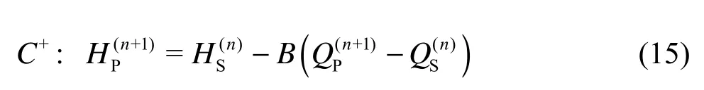
where B=a/(gA), g is the acceleration of gravity, and A is the area. The head loss is ignored because the distance between nodes S and P is very short.

Ruprecht[10,11]proposed a coupling method, in which the head at the Section 1-1 at the time step n is substituted for that at the node P(n+1)at the next time step to solve Eq.(15). The process is as follows:

(1) As shown in Fig.1(a), the variables of the 1-D and 3-D grids are assumed to be known at the time step n, then construct the+C equation Eq.(15) between nodes S and P(n+1).

(2) Calculate the average headat the Section 1-1 of the CFD boundary.

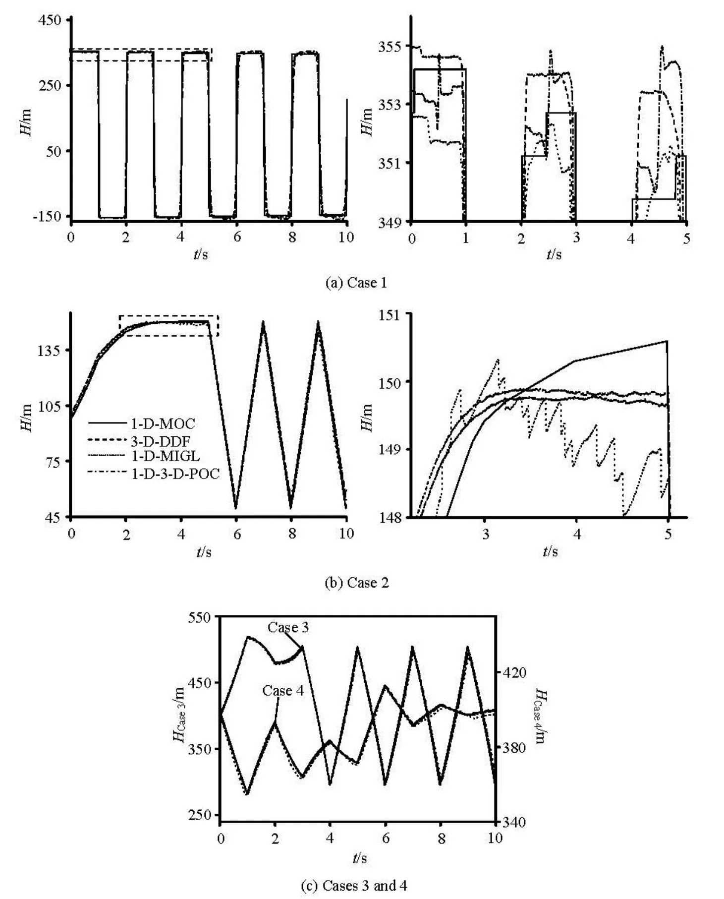
Fig.2 Histories of the head at the valve

(5) Calculate the average headat the Section 1-1 at the boundary of the CFD grid.

This method is relatively simple to formulate and program, and involves the influence of the water hammer waves in the pipe system on the discharge at the 3-D CFD boundary, inthe simulation ofthe p ressure fluctuationsin the draft tube[10,11]and the runaway process of aturbine[12]. However, itinvolves the assumption that=, which may not be valid if the difference in the heads between adjacent time steps varies sharply, so the time step must be small enough.

Fig.3 Schematic layout of a simple surge tank

2.2 New coupling methods

To obtain the head and the discharge at the node P(n+1), we can construct an auxiliary equation to specify the relationship betweenand. Two methods are presented.

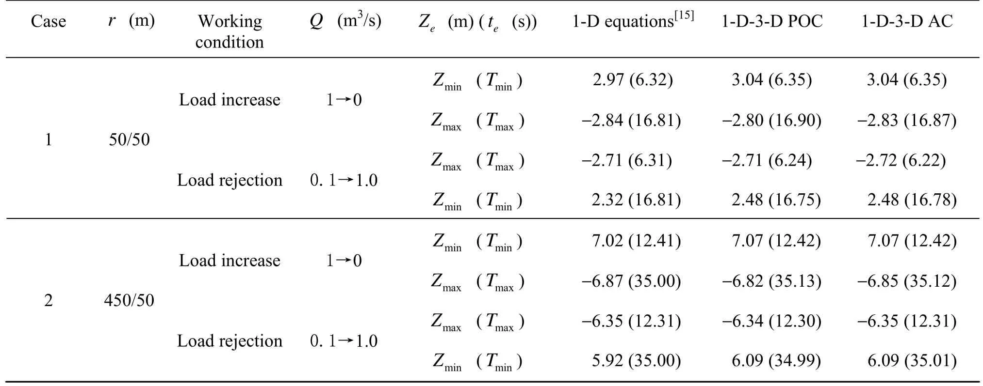
Table 2 Calculated cases and results of the surge tank surge waves simulation

2.2.1 Partly Overlapped Coupling (POC)

A section of the 3-D CFD grid is considered as the 1-D MOC grid and construct the C-equation (Eq.(16)) at the right side of the node P(n+1)

The node P is no longer the downstream boundary of the 1-D part but is still the upstream boundary of the 3-D part, and it appears as if the 1-D MOC grid extends to the 3-D CFD grid, as shown in Fig.1(b). The downstream point M of the extended MOC grid boundary is located in the internal Section 2-2 of the CFD grid, and therefore, it is called the partly overlapped coupling method. The process is as follows:

(1) As shown in Fig.1(b), the flow variables in the 3-D part are assumed to be known at the time step n.

(2) Calculate the average headand dischargeat the Section 2-2 of the CFD grid at the time step n.

(4) Construct the C+equation (Eq.(15)) between the nodes S and P(n+1)and the C-equation (Eq.(16)) between the nodes M and Pn+1, then combine the two equations and solve forand.

This method models a section of the MOC grid using the CFD grid, which is clear in the physical meaning and simple in the procedure.

2.2.2 Adjacent Coupling (AC)

In Fig.1(a), consider a section of the CFD grid (Section 1-2) on the right side of the node P as a 1-D domain and the flow can then be expressed by the unsteady Bernoulli equation, expressed as

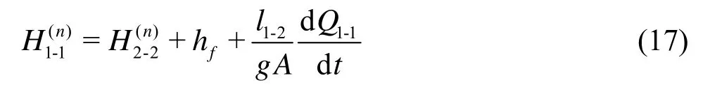
where1-2l is the length of the Section 1-2,fh is the head loss and can be ignored here. Substitute the derivative with the difference to give

where Δt is the time step. The head and the discharge at the node P(n+1)can be obtained by solving Eq.(18) combined with the C+equation (Eq.(15)). Here, the 1-D and 3-D grids are adjacent to each other, so the method is called the adjacent coupling method. The process is as follows:

(1) As shown in Fig.1(a), the flow variables of the 1-D and 3-D parts are assumed to be known at the time stepn, we can then construct the C+equation (Eq.(15)) between the nodes S and P(n+1).

(2) Calculate the average headand the dischargeat the Section 1-1 of the CFD grid at the time step n.

(3) Calculate the average dischargeat the Section 2-2 of the CFD grid at the time step n.

This method is similar to that of Ruprecht’s in the arrangement of the grids of the two parts, but there is no assumption here and it has a more explicit physical meaning. However, the procedure is a little more complex than the POC method. The accuracy of these two methods will be compared in the next section.

3. Verifications

3.1 Water hammer waves

To validate the methods for modeling the compressible water proposed above, the 1-D water hammer waves are simulated using the 3-D methods. Consider a piping system with a reservoir upstream and a valve at the downstream end, of 500 m in length and 4 m2in cross-sectional area. With the speed of sound a0=1000m/s and the coefficient of friction resistance λ=0.014 in the MOC, and other computational conditions listed in Table 1, the 1-D MOC, the 3-D DDF, the 3-D MIGL and the 1-D-3-D POC methods are applied to simulate four types of water hammer waves. Note that in the coupling case, the POC method is used; the lengths of the 1-D and 3-D parts are equal and the water compressibility in the 3-D domain is modeled by the DDF.

Figure 2 illustrates comparisons of the heads at the valve between the two 3-D methods and the MOC for the four types of water hammer waves. The curves for the DDF and MIGL agree well with those of the MOC. Table 1 presents the values of the extreme heads and their occurrence times. The maximum error of the extreme heads between the two methods proposed here and the MOC is 2.9 % relative to the initial heads. The maximum deviation for the occurrence times is less than 3.0 % for Cases 3 and 4 relative to the period of the waves. However, the figure is much larger for Cases 1 and 2, because there are fluctuations within the narrow ranges in the head curves (see Figs.2(a) and 2(b)) especially in the 3-D MIGL simulations. However, the average values agree well with the results of the MOC. In addition, the results of the 1-D-3-D POC also indicate that it is proper to simulate the MD water hammer using the 1-D-3-D coupling method with the DDF method in the 3-D part. It is clear that the two methods are both valid while the stability of the results of the DDF is better than that of the MIGL.

3.2 Oscillations of the water level in the surge tank

To validate the 1-D-3-D coupling methods, the 1-D water level oscillations in the surge tank are simulated here. Figure 3 shows a typical simple surge-tank system and the cross-sectional area of the water conveying tunnel is equal to that of the tank. We use the 1-D surge tank governing equations[15], the 1-D-3-D POC and AC methods to simulate the load increase and the rejection processes, which are all completed in 2.0 s. Table 2 shows two cases, which differ both in the total length and the ratio of the 1-D and 3-D parts.

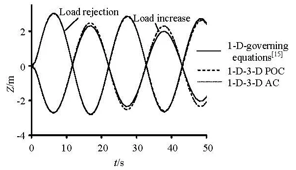
Fig.4 Oscillations of the water level for Case 1

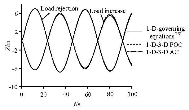
Fig.5 Oscillations of the water level for Case 2

Figures 4 and 5 compare the oscillations of the water level obtained by the two 1-D-3-D coupling methods proposed above and the 1-D governing equations. There is no visible difference between the results obtained with the two coupling methods. Their wave shapes agree well with those of the 1-D results but with slower damping. Table 2 displays the extreme amplitudes of the oscillations and their occurrence times, and the maximum deviations of the extreme

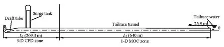
Fig.6 Schematic diagram of the completely computational domain

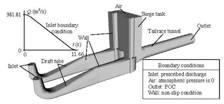
Fig.7 Schematic diagram and boundary conditions of the 3-D computational domain

amplitudes obtained by the two coupling methods with respect to the 1-D data are less than 6.9% for Case 1 and 2.9% for Case 2. Meanwhile, the maximum deviation for the occurrence times is not larger than 0.45 % relative to the oscillation periods for the two cases. It should be noted that the damping process of the oscillation is not sensitive to the length of the system, but the period is only decided by the length provided the cross-sectional areas of the tunnel and the tank are fixed. Therefore, according to the accurate predictions of the occurrence times of the extreme values, it is reasonable to conclude that the two coupling methods proposed here are valid and accurate in the same degree,

4. Simulation of the transients in a hydropower system

4.1 Computational conditions

The hydropower system considered in this simulation adopts the tailrace layout of two turbines, one surge tank and one tailrace tunnel. The two branches and the main tailrace tunnels are connected by an asymmetrical bifurcation. Figure 6 illustrates schematically the complete computational domain. The tailrace surge tank is an orifice that is connected at the top and separated at the bottom (see Fig.7). To estimate the flow patterns in the existing surge tank geometry at the lowest water level, the load rejection process for all the turbines in a unit with the lowest tailrace water level of 25.9 m is simulated using the 3-D CFD method. The tailrace tunnel is relatively long, so the 1-D-3-D coupling approach is applied here.

As shown in Fig.6, the complete computational domain has a length of 209.3 m for the 3-D part and 640.0 m for the 1-D part. The 3-D CFD domain and the boundary conditions are shown in Fig.7, but only half of it is used for the simulation because of its symmetrical features. For the inlet of the draft tube, the prescribed discharge, decreasing with time, is provided. For the 1-D-3-D coupling, the POC is preferred, which would let the wave propagate with no reflection, and is used. The VOF model is applied to track the free surface. For the turbulence treatment, the RNG kε- model is adopted.

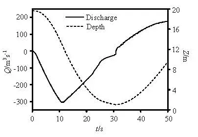
Fig.8 Histories of the discharge and the submerged depth of the existing geometry

4.2 Results and analyses

During the load rejection process, the discharge from the draft tube gradually reduces to zero. Meanwhile, the water in the tailrace tunnel keeps movingdownstream due to inertia, therefore, the water surface immediately falls to a minimum level in the surge tank. In such a case, if the submerged depth relative to the tank bottom is significantly low, some harmful flow patterns will appear, such as the air-entrained vertical vortex or the air suction into the tailrace tunnel.

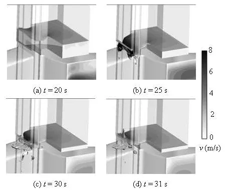
Fig.9 Flow patterns of the existing geometry (half part only, colored by velocity magnitude)

Figure 8 depicts the histories of the discharge into the tank and the submerged depth relative to the tank bottom for the existing geometry. The minimal submerged depth is approximately 1.0 m at about 30.0 s, which is the lowest value according to the design requirement. Correspondingly, the fact that the value for the discharge drops off considerably at about the same time can be explained by the flow patterns as shown in Fig.9. It is obvious that at this moment, the water level around the orifice falls to the elevation under the tank bottom and a large volume of air is brought into the tailrace tunnel, which will definitely damage the tunnel structure. Therefore, a modification is needed for the existing geometry.

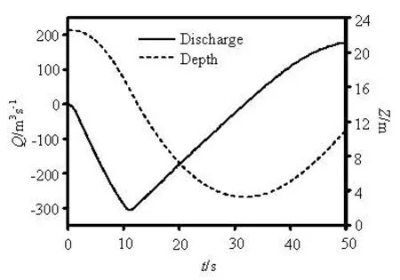
Fig.10 Histories of the discharge and the submerged depth of the modified geometry

A method of reducing the elevation of the tank bottom by 3.0 m is adopted in the existing geometry. The simulated histories of the discharge into the tank and the submerged depth relative to the tank bottom are depicted in Fig.10. The discharge varies smoothly, and the minimal submerged depth is more than 3.0 m. Figure 11 shows the flow patterns of the modified geometry and it is clear that the water surface is relatively stable under the condition for the lowest level satisfying the design requirement.

Fig.11 Flow patterns of the modified geometry (half part only, colored by velocity magnitude)

5. Conclusions

Two methods for modeling the compressible water with the CFD software and two treatments for coupling 1-D and 3-D computational domains are proposed in this paper. The load rejection process of a hydropower system is simulated by the 1-D-3-D POC method. The conclusions are as follows:

(1) The methods of the DDF and the MIGL for modeling the compressible water presented here are both valid and accurate enough to predict the characteristics of the typical water hammer waves, and can be applied in practical applications. The DDF is considered a better method than the MIGL both in terms of the physical interpretations and the stability of the results.

(2) The methods of the POC and the AC for coupling the 1-D and 3-D computational domains proposed above are both valid and accurate while the procedure of the POC is marginally simpler than that of the AC method.

(3) The 1-D-3-D coupling approach is an efficient and promising way to simulate the hydraulic transients in the hydropower systems in which the interactions between 1-D hydraulic fluctuations of the pipeline systems and the local 3-D flow patterns should be considered.

This paper presents preliminary results of simulating MD transients in hydropower systems. Somefuture work will include:

(1) An implicit method for modeling the compressible water is to be developed to solve complicated problems with larger time step.

(2) Further studies will focus on the coupling multiple 3-D domains, such as surge tanks and turbines, with respect to the 1-D water conveying system.

[1] POPESCU M., ARSENIE D. and VLASE P. Applied hydraulic transients for hydropower plants and pumping stations[M]. Rotterdam, The Netherlands: A. A. Balkema, 2003.

[2] CHANG Jin-shi. Transients of hydraulic machinery[M]. Beijing: Higher Education Press, 2005, 7-10(in Chinese).

[3] YANG Jian-dong, ZHAO Kun and LI Lin et al. Analysis on the causes of units 7 and 9 accidents at Sayano-Shushenskaya Hydropower Station[J]. Journal of Hydroelectric Engineering, 2011, 30(4): 226-234(in Chinese).

[4] CHENG Yong-guang, SUO Li-sheng. Lattice Boltzmann scheme to simulate two-dimensional fluid transients[J]. Journal of Hydrodynamics, Ser. B, 2003, 15(2): 19-23.

[5] KOLŠEK T., DUHOVNIK J. and BERGANT A. Simulation of unsteady flow and runner rotation during shutdown of an axial water turbine[J]. Journal of Hydraulic Research, 2006, 44(1): 129-137.

[6] CHENG Yong-guang, LI Jin-ping and YANG Jiandong. Free surface-pressurized flow in ceiling-sloping tailrace tunnel of hydropower plant: Simulation by VOF model[J]. Journal of Hydraulic Research, 2007, 45(1): 88-99.

[7] YAN J., KOUTNIK J. and SEIDEL U. et al. Compressible simulation of rotor-stator interaction in pump-turbines[C]. 25th IAHR Symposium on Hydraulic Machinery and Systems. Timisoara, Romania, 2010.

[8] LIN Ching-long, TAWHAI H. and MCLENNAN G. et al. Multiscale simulation of gas flow in subject-specific models of the human lung[J]. IEEE Engineering in Medicine and Biology Magazine, 2009, 28(3): 25-33.

[9] HAN Dong, FANG Hong-wei and BAI Jing et al. A coupled 1-D and 2-D channel network mathematical model used for flow calculations in the middle reaches of the Yangtze River[J]. Journal of Hydrodynamics, 2011, 23(4): 521-526.

[10] RUPRECHT A., HELMRICH T. and ASCHENBRENNER T. et al. Simulation of vortex rope in a turbine draft tube[C]. 21st IAHR Symposium on Hydraulic Machinery and Systems. Lausanne, Switzerland, 2002.

[11] RUPRECHT A., HELMRICH T. Simulation of the water hammer in a hydro power plant caused by draft tube surge[C]. 4th ASME/JSME Joint Fluids Engineering Conference. Honolulu, Hawaii, USA, 2003.

[12] CHERNY S., CHIRKOV D. and BANNIKOV D. et al. 3D numerical simulation of transient processes in hydraulic turbines[C]. 25th IAHR Symposium on Hydraulic Machinery and Systems. Timisoara, Romania, 2010.

[13] GHIDAOUI S., ZHAO M. and MCLNNIS A. et al. A review of water hammer theory and practice[J]. Applied Mechanics Reviews, 2005, 58: 49-76.

[14] WU Wang-yi. Fluid mechanics[M]. Beijing: Peking University Press, 2009, 171-179(in Chinese).

[15] LIU Qi-zhao, HU Ming. Hydropower station[M]. 4th Edition, Beijing: China Water Power Press, 2010, 214-216(in Chinese).

10.1016/S1001-6058(11)60282-5

* Project support by the National Natural Science Foundation of China (Grant Nos. 51039005, 50909076).

Biography: ZHANG Xiao-xi (1986-), Male, Ph. D. Candidate

CHENG Yong-guang,

E-mail: ygcheng@whu.edu.cn