How do the landslide and non-landslide sampling strategies impact landslide susceptibility assessment? -A catchment-scale case study from China
2024-03-25ZizhengGuoBixiTinYuhngZhuJunHeTiliZhng
Zizheng Guo,Bixi Tin,Yuhng Zhu,Jun He,Tili Zhng
a School of Civil and Transportation Engineering, Hebei University of Technology, Tianjin, 300401, China
b Hebei Key Laboratory of Earthquake Disaster Prevention and Risk Assessment, Sanhe, 065201, China
c Faculty of Engineering, China University of Geosciences, Wuhan, 430074, China
d Nanjing Center, China Geological Survey, Ministry of Natural Resources, Nanjing, 210016, China
Keywords: Landslide susceptibility Sampling strategy Machine learning Random forest China
ABSTRACT The aim of this study is to investigate the impacts of the sampling strategy of landslide and non-landslide on the performance of landslide susceptibility assessment(LSA).The study area is the Feiyun catchment in Wenzhou City,Southeast China.Two types of landslides samples,combined with seven non-landslide sampling strategies,resulted in a total of 14 scenarios.The corresponding landslide susceptibility map(LSM) for each scenario was generated using the random forest model.The receiver operating characteristic(ROC)curve and statistical indicators were calculated and used to assess the impact of the dataset sampling strategy.The results showed that higher accuracies were achieved when using the landslide core as positive samples,combined with non-landslide sampling from the very low zone or buffer zone.The results reveal the influence of landslide and non-landslide sampling strategies on the accuracy of LSA,which provides a reference for subsequent researchers aiming to obtain a more reasonable LSM.
1.Introduction
Landslides are one of the major geological disasters all over the world,causing considerable human casualties and economic losses every year (Petley,2012).For example,the southeastern part of China often suffers from rainstorm-triggered landslide events in summer,which may lead to dozens of deaths and millions in economic losses(Su et al.,2015;Zhao et al.,2019;Ma et al.,2022a;Guo et al.,2023a).Thus,spotting the areas exposed to landslides is an important task for land planning and regional security(Chen and Li,2020;Guo et al.,2020a).Recently,landslide susceptibility mapping(LSM) has been a commonly used tool for achieving this goal,and extensive stakeholders have begun to assess and reduce landslide risk through it(Brenning,2005;van Westen et al.,2008;Agterberg,2022).
Landslide susceptibility assessment(LSA)is to obtain the spatial distribution of landslide occurrence probability in a region by analyzing the correlation among historical landslides and environmental factors (Fell et al.,2008;Pradhan,2010).A normal LSA procedure mainly includes the sampling of landslides (positive)and non-landslide (negative) datasets,and the determination of influencing factors,landslide susceptibility modelling and mapping,and accuracy analysis of results (Barik et al.,2017).Among them,input data commonly differs in terms of landslide and nonlandslide samples,leading to a significant source of uncertainty in LSA.Specifically,it is important to accurately express the spatial shape of landslide samples and the spatial location of non-landslide samples because they can affect the nonlinear correlation between samples and factors during modelling,which further impacts the accuracy of LSA (Arnone et al.,2016).
The landslide locations are usually determined from historical landslides,remote sensing images,and field investigations(Guzzetti et al.,2012;Guo et al.,2020b;Smith et al.,2021).Then the landslides should be digitized for the analysis of the relationship between landslides and environmental factors (Peng et al.,2014;Paryani et al.,2021).At present,expression forms of landslide samples in the literature mainly include points (Guo et al.,2022),circles (Huang et al.,2022) or irregular shapes (dustpan shapes,semicircles,elongated bars,etc) (Galli et al.,2008;Moosavi et al.,2014).Specifically,the selection of landslide digital form largely depends on the study scale and landslide size.For studies at small scales (1:100,000 or smaller),it is commonly an operational challenge to accurately capture the actual boundary of landslides thus the forms of point and circle are mainly adopted under this condition (van Westen et al.,2006).Users only need to record limited but necessary information on landslides (e.g.,location,type,and time) in the inventory.At medium (1:10,000-1:50,000) or large scales (>1:50,000),more information can be revealed in the landslide inventory since the test area is smaller,allowing for more detailed investigations,including initiation area,accumulation area,size and abundance.It is also common to identify the actual boundaries (irregular shapes) of landslides,especially with the development of remote sensing and drone techniques (Azarafza et al.,2018;Nikoobakht et al.,2022;Su et al.,2022).Considering the systematic error when it comes to the form of landslide points and circles,more studies prefer to digitalize the landslides as irregular shapes for the LSA (e.g.,Shahabi and Hashim,2015;Ma et al.,2022b),which align more closely with realistic situations.As Huang et al.(2022)pointed out,landslide samples expressed by irregular shapes (actual boundary) often have a higher result accuracy and a lower uncertainty in landslide susceptibility modelling.When a landslide inventory with irregular shapes is used for LSA,a data transformation from vector to raster(pixel)is required.However,when landslides are represented in GIS by pixels,their boundaries and pixel boundaries often do not completely overlap.There is not yet a unified standard determining whether a pixel crossing a landslide boundary should be considered part of the landslide samples.Although this aspect may significantly impact the outcome of the susceptibility analysis,the issue of the proper representation of landslide locations has not been widely discussed yet.
Regarding the sampling strategy of non-landslide dataset,there are mainly four kinds of ways: (i) sampling randomly from landslide-free areas,which is the most commonly used one in the literature (e.g.Okalp and Akgün,2016;Bueechi et al.,2019;Azarafza et al.,2021),(ii)sampling from the buffer zone by defining a minimum distance between the landslide area and a landslidefree area (Xi et al.,2022),(iii) sampling from the low susceptibility zone obtained by constraining certain external factors,such as self-organizing neural network (Huang et al.,2017),similaritybased approach (Zhu et al.,2019),and (iv) sampling from terrain area with low slope angles or plain regions (Kavzoglu et al.,2014;Lucchese et al.,2021;Okalp and Akgün,2022).However,all these strategies have inherent drawbacks which can cause some important aspects of uncertainty to the LSA (Zhu et al.,2019).For example,the negative samples generated by (i) and (ii) may be located on steep slopes that are susceptible to landslides.The strategy (iv) may identify the pixels near rivers which are also possibly prone to landslide occurrence.Hence,it is necessary to compare and assess the performance of different sampling strategies of non-landslide dataset in the LSA.Unfortunately,limited efforts have been made on this issue.Xi et al.(2022)compared the results from two scenarios,namely a set of negative samples created using different buffer distances (strategy (ii)) and a set of negative samples created by the Newmark-based method(strategy(iii)).Except this,more studies simply propose a specific method for non-landslide sampling and test its performance.The uncertainty stemming from this aspect remains due to the lack of comprehensive comparisons among different scenarios.
The commonly-used models for LSA can be divided into expertbased models(Sezer et al.,2017),physically-based models(Medina et al.,2021)and data-driven models(Eker et al.,2015;Zêzere et al.,2017).Generally,data-driven models can be classified as statistically-based and machine learning models(Pham et al.,2016;Reichenbach et al.,2018;Guo et al.,2023b).Compared with mathematical statistics,machine learning models have advantages in reflecting the nonlinear corrections between landslides and factors(Bueechi et al.,2019).Thus,models like Random Forest(RF),C5.0 Decision Trees (C5.0 DT),Logistic Regression (LR),Bayes Network (BN),Artificial Neural Networks (ANN),Multilayer Perceptron (MLP) and Support Vector Machine (SVM) have been widely developed and applied for LSA over the past decade (Bui et al.,2012;Conforti et al.,2014;Hong et al.,2020;Merghadi et al.,2020).Additionally,some recent advances in data processing techniques show that ensemble learning methods can further improve the performance of machine learning methods and alleviate their limitations (e.g.Bui et al.,2019;Chen and Li,2020).However,it should be noted that a sole type of machine learning model may be coincidental regarding high accuracy,so it is necessary to consider different models to obtain more stable and reliable results.In this study,we used three models including C5.0 model,SVM LR models to generate landslide susceptibility maps,which herein we refer to as pre-LSM.The non-landslide dataset was sampled from the very low susceptibility zones in these pre-LSMs,which was subsequently used to generate final LSM.Considering the high accuracy and maturity of the RF model(Catani et al.,2013),this model was selected for the final landslide susceptibility modelling.
In general,the application of machine learning in the field of LSA is relatively mature.However,there are imperfections in the modelling process.Specifically,there is limited research on the gridding method for landslide datasets and the selection of nonlandslide samples.The main objective of the present study is to clarify the uncertainties from landslide and non-landslide sampling strategy and reveal their impacts on LSA.As far as we know,very few studies have discussed the combined effect of both aspects before.The Feiyun catchment in Zhejiang Province of Southeast China was taken as the study area.More specifically,our aims include: (i) design of landslide and non-landslide sampling strategies based on various sampling areas;(ii) constructing the combined scenarios of sampling strategies and conducting regional LSA based on machine learning models;and (iii) comparative analysis of predictive ability under different scenarios and effects of sampling strategies.
2.Materials
2.1.Study area
The present study was conducted in the Feiyun catchment,which is located southwest of Wenzhou,Zhejiang Province,China.It covers a total area of 388.17 km2and is geographically between latitudes 119°59′32′′E and 120°15′30′′E,longitudes 27°39′12′′N and 27°50′29′′N (Fig.1).The landscape of the region is dominated by mountains and hills,and the elevation ranges from 12 m above sea level at the river valley to 1091 m at the highest peak,with the topography characterized by higher elevation in the northwest and lower elevations in the southeast.The area is a subtropical marine monsoon climate zone with a multi-year average temperature of 14°C-18.5°C and a multi-year average rainfall of approximately 1884.7 mm.The river systems in the area are well developed,with the Feiyun River being the main stream which flows through the catchment from west to east,and the settlements are mainly located along the river banks.The predominant strata outcrops in the region comprise volcanic rock,granites,Paleozoic clastic rock,and carbonate rock(Su et al.,2015;Wang et al.,2020).
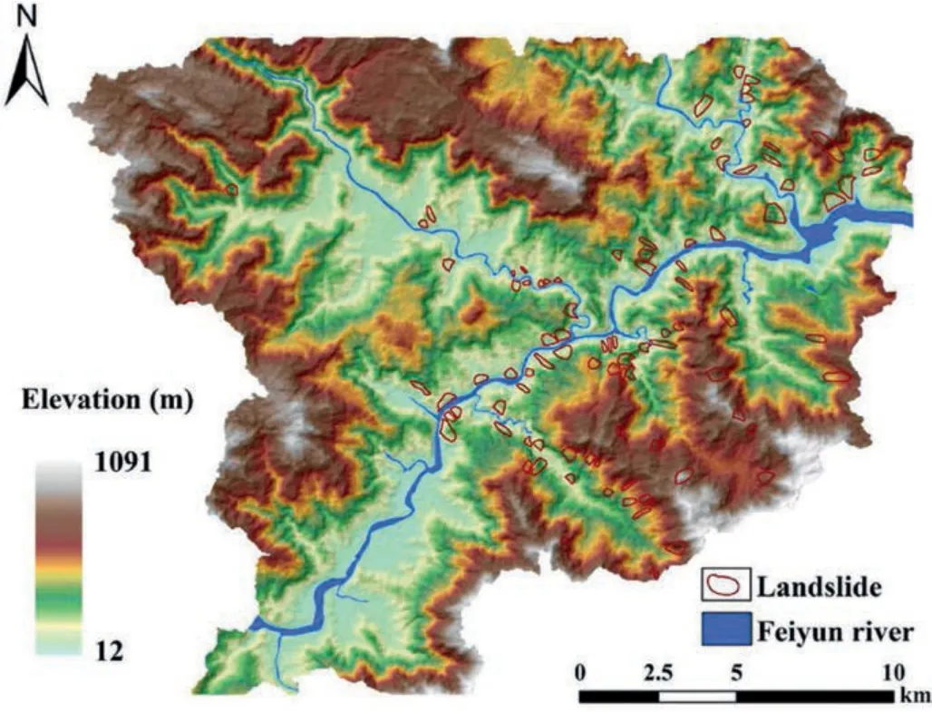
Fig.1.Distribution of the landslides in the study area where the DEM with a resolution of 30 m is used as the base map.
2.2.Landslide inventory
The LSA by applying data-driven models is commonly based on an important assumption that future landslides will likely occur in areas with environments similar to those of historical landslides(Zêzere et al.,2017).Therefore,landslide inventory as a basis for understanding the spatial distribution of historical landslides in a region is essential (Huang et al.,2017).In this study,based on historical landslide reports,visual interpretation of remote sensing images and field geological surveys,96 landslide points are identified in the inventory(Fig.1).Their boundaries were also identified and subsequently digitized as polygons.Covering a total area of 8.8 km2,these landslides constitute 0.23% of the total study area.These landslides are mainly developed along the river banks of the central and northwestern part,and identified as shallow type according to Varnes classification system(Varnes,1978;Hungr et al.,2014).The most important triggering factor for them is heavy rainfall in rainy season,which commonly happens with typhoon events.
2.3.Data source and preparation of influencing factors
The data used in this study mainly includes the digital elevation model(DEM),satellite images,the survey map of the study area and water system.Detailed information and the purpose of the data are shown in Table 1.
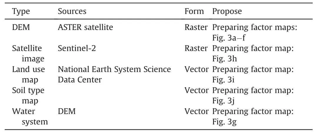
Table 1 The information of data used in this study.
The development and mechanism of landslides over a large area are complex and diverse,and mainly influenced by five types of factors,namely topography,hydrology,land cover,geology and others(e.g.human engineering activities)(Reichenbach et al.,2018;Goyes-Penafiel and Hernandez-Rojas,2021).There is no agreement on the best combination of influencing factors for LSA so far.In this study,ten factors (Fig.2) were selected for analysis,based on previous literature and overall characteristics of landslides in the region.It should be stated that the rainfall was not taken into account in this study because it was considered relevant to temporal probability of landslides,which was beyond the concept of landslide susceptibility in the widely accepted criterion (Fell et al.,2008).

Fig.2.The influencing factors used for:(a)Aspect,(b)Elevation,(c)Slope,(d)Relief,(e)Profile curvature,(f)TPI,(g)Distance from river,(h)NDVI,(i)Land cover,and(j)Soil type.
Topographic factors include aspect,elevation,slope,topographic position index (TPI),profile curvature and relief.Among them,slope is considered as the most important topographic factor that can directly control slope stability (Zhou et al.,2016).Aspect and TPI orientation indirectly affect landslide development by influencing the vegetation distribution and illumination of the slope (He et al.,2019).Elevation reflects the changes of the temperature,humidity and biodiversity on the slope (Shahri et al.,2019).Relief and profile curvature characterize the undulation of the terrain and subsequently control the water flow on the slope surface.The degree of relief was obtained by searching the 3 m × 3 m neighborhood grid unit and calculating its maximum elevation difference.The other factors were all generated by digital elevation model (DEM) data with spatial resolution of 30 m in GIS 10.6 software.
The hydrological factor was represented by the distance from the river,because it can affect groundwater level,drainage capacity of slopes and erosion on the bank slopes.Therefore,with the drainage line as the buffer center and 100 m intervals from 0 to 600 m,six equally spaced buffer zones were determined.Combined with the areas with the distance to river beyond 600 m,a total of seven levels were generated to represent the impact range of the river on the bank slopes.
Land cover influences the infiltration,drainage and antiweathering ability of slopes,thus causing instability (Dao et al.,2020).The land cover data were downloaded from National Earth System Science Data Center (https://www.geodata.cn).It was divided into eleven categories,namely,dense forest,open forest,garden,shrubs,dense grass,open grass,paddy field,dry land,bare land,urban area and water,which were remarked from 1 to 11 in order.Moreover,normalized difference vegetation index (NDVI)was also considered,which can reflect the development of vegetation.Vegetation roots can reinforce soil and slow down soil erosion.Compared with densely vegetated areas,bare slopes without vegetation cover are commonly more prone to deformation when exposed to external conditions such as rainfall(Hürlimann et al.,2022).This map was calculated by using Sentinel-2 images at different wavelengths.
Geological factors are crucial in controlling landslide materials.Different soil types have various mechanical and hydrological properties,which have significant effects on occurrence of shallow landslides.Since most landslides in the study area were identified as shallow types,soil type was considered as geological factor.The soil type factor was obtained from National Earth System Science Data Center (https://www.geodata.cn),and it was divided into six types including red soil,yellow soil,paddy soil,submergic paddy soil,acid soil and brown soil,which were remarked from 1 to 6 in order.According to Chinese Soil Taxonomy,different soil types present different colors due to the difference of soil textures,so the colors can be used to represent soil type (Liu et al.,2020).
3.Methodologies
3.1.Modelling procedure
The flow chart of this study is shown in Fig.3.Overall,there are totally five main steps as follows: (i) Data preparation and factor reclassification: All influencing factors were generated into raster with a resolution of 30 m using ArcGIS.Among these influencing factors,seven are continuous variables except for distance from river,land cover and soil type,which are discrete.On one side,it is time-consuming if every single value of the variables is used as the input parameter for the model without the division of classes.On the other side,a relevant source of subjectivity and uncertainty is introduced when splitting the input parameters into fixed classes with a certain of break values.To resolve this issue,the continuous influencing factors were first equally classified into 20 subcategories,and then the frequency ratio of each classification was calculated in this study.Finally,the sub-categories with similar frequency ratios were grouped to form the final influencing factor classification.It should be mentioned that the final arbitrary number of classes was determined from 5 to 7,which fits with previous studies(Dou et al.,2020;Huang et al.,2020).The details of frequency ratio analysis for each factor will be described in section 4.1: (ii) Landslide sampling strategy: Two landslide expression styles were designed in this part.One is the rasters only within the landslide boundary (herein we call it by “landslide core”) were considered as the landslide dataset after rasterization of the landslide surface.The other one is that the rasters including landslide core and the rasters covering the landslide boundary were integrated as the entire group (herein we call it by “landslide extension”) (see the “sampling strategy” section for the detailed definitions of landslide core and landslide extension).(iii) Nonlandslide sampling strategy: Seven scenarios were determined to sample non-landslide datasets,which can be divided into three categories.The first one was sampling non-landslides from landslide-free areas,which was commonly used in literature (Ali et al.,2022;Mehrabi,2022).The second one was to obtain nonlandslide samples from the buffer zone (within the distance of 200 m,200-400 m,and larger than 400 m buffer zone to landslide boundary,respectively).The third method was to sample nonlandslides from the very low susceptibility zones identified by some models in advance(herein we call it pre-LSM).Three machine models were applied to create pre-LSMs in this study,namely SVM,C5.0 and LR models.(iv) LSM: A total of fourteen scenarios were determined by combining the landslide and non-landslide sampling strategies mentioned above,and the LSM under each scenario was generated based on the RF model.(v) Validation and comparison: The receiver operating characteristic (ROC) curve and area under curve (AUC) value for each scenario were calculated to analyze the model performance and evaluate the effect of sampling strategy on LSA.It should be stated that three different machine learning models were employed in step(iii)to mitigate the chance of incidental errors in VL zone produced by a single model.During step(iv),the purpose of the application of the RF model instead of the three models mentioned above was to keep the sampling of landslide/non-landslide as the only variable in the test.The details on the model principles used will be described in continuation.
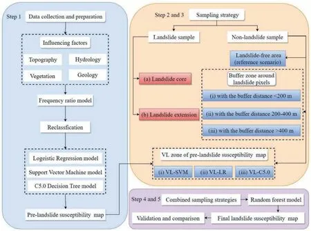
Fig.3.The methodological framework of this study.
3.2.Frequency ratio (FR) model
The frequency ratio(FR)method is a traditional statistics model for regional LSA.The FR values of one factor greater than 1 indicate a positive relationship with landslide occurrence,and conversely FR values less than 1 represent a negative relationship (Shirzadi et al.,2017).It is now commonly used for the grading of influencing factors:
whereiandjindicate the number and grading of impact factors respectively,Lijindicates the area of landslides within classjof theith influencing factor andTLrepresents the total area of landslides;Cijindicates the area of classjof theith impact factor andTCrepresents the total area of the study area.
3.3.Machine learning models
3.3.1.C5.0 decision tree(C5.0 DT)
The C5.0 Decision Tree model is based on a multistage or hierarchical decision structure.The core of the C5.0 DT model is using the rate of decline in information gain ratio (GR) as the basis for determining the optimal branching variables and segmentation thresholds.The GR can be expressed as following(Guo et al.,2021):
whereDis the dataset andTis the predictor variable.TheGains(D,T)represents the entropy difference between the original and child nodes,which is calculated as below:
whereCis the target variable,nis the category number ofC,Ci(i=1,2,…,n).The category number ofTism,Tj(j=1,2,…,m).In this study,Adaboosting algorithm and Pruning was adopted to improve the generalization ability of the C5.0 DT model during the modelling process.
3.3.2.Support vector machine(SVM)
The SVM model is a sparse and robust classifier that uses a hinge loss function to compute empirical risk and adds a regularization term to the solution system to optimize structural risk.The SVM model is one of the common kernel learning methods for nonlinear classification by the kernel method(Zhang et al.,2019).Generally,a high-dimensional feature space was map data through nonlinear kernels and classified by separating hyperplane.The separating hyperplane can be defined as following:
with the optimal solution to:
where ω determines the direction of the hyperplane,bis the bias,Crepresent the penalty,xi∊Rn,yi∊{-1,1},ξiis the slack factor used for classifier and the number of support vectors is l.The classification function is calculated as Eq.(7) by introducing kernel functions:
wherenis the number of the samples,andaiis Lagrange multiplier.
3.3.3.Logistic regression(LR)
The logistic regression method is a classic linear regression model that has been widely applied to solve dichotomous problems in LSA(Kavzoglu et al.,2014).The main calculation formula of it can be written as following:
wherezis the linear predictor for landslide,y nis the characteristic value of influencing factors,kis a constant anda nis thenth regression coefficient.The weighted values of each influencing factor were obtained by the product ofyn(characteristic value)anda n(coefficient) of each influencing factor.And the landslide susceptibility index (IS) can be calculated as
3.3.4.Random forest(RF)
The RF model is an integrated learning method that combines multiple decision trees for classification and prediction.The classifier is a recursive process from the root node to the child nodes,selecting a random portion of samples and features from the training data with put-backs(Ilia et al.,2018;Dou et al.,2019).From the nodes of the tree,branches are determined based on the optimal features between the nodes,and branching is continued until the result of a tree is obtained.Finally,the subset of categories with the most votes can be selected as the final outputs:
whereT(X)is the combined classification model,each node is denoted bykandtiis the decision tree.The output variable and the feature function are represented byUandI.The marginal function can be denoted by the following equation:
The classification reliability of the model is proportional to the value of the function.The following equation is principle of the categorization:
where (X,U) is the probability space andPrepresents the feature variable.
The model does not require any transformation or rearrangement for disaggregated data,thus can effectively eliminate overfitting of data Considering it has strong generalization ability and high accuracy,the RF model has been widely used in the topic of LSA(Kim et al.,2018;Hong et al.,2019).The RF generally consists of two trees(positive and negative),each of which was constructed by using ten random features (influencing factors) in this study.The purpose of this study is to explore the impact of sampling strategies on LSA,so using a stable model can reduce the effect of uncertainty from the model itself.This is the reason why the RF model was used as the approach to generate final landslide susceptibility maps.
3.4.Sampling strategy
3.4.1.Landslide sampling strategy
The conversion of landslide inventory from vector to raster is a delicate operation when conducting landslide susceptibility modelling.Different rasterization methods impact the calculation of landslide area which may result in large differences in landslide information.Moreover,the landslide shape,area and raster resolution also influence the final results,especially when the landslide area is small and the raster resolution is coarse(Arnone et al.,2016;Huang et al.,2022).When the number of pixels involved in the landslide boundary is large,whether to consider the landslide boundary pixels as the landslide sampling dataset may have a large impact on the landslide information included into the model.Hence,two landslide rasterization scenarios (landslide core and landslide extension) were designed to evaluate the influence of rasterization methods.Usually,the landslide boundary occupies one pixel,and sometimes up to two pixels (Fig.4a).The landslide core was expressed by all the pixels contained in the landslide boundary and was obtained through the Polygon to Raster tool in GIS 10.6 software as shown in Fig.4b.The landslide extension was the pixels combination of landslide core and landslide boundary(Fig.4c).In this study,the landslide boundary includes 4161 pixels,the landslide core contains 9805 pixels,and the landslide extension contains 13966 pixels.The ratio of landslide boundary to core is 0.424 under the raster resolution of 30 m.
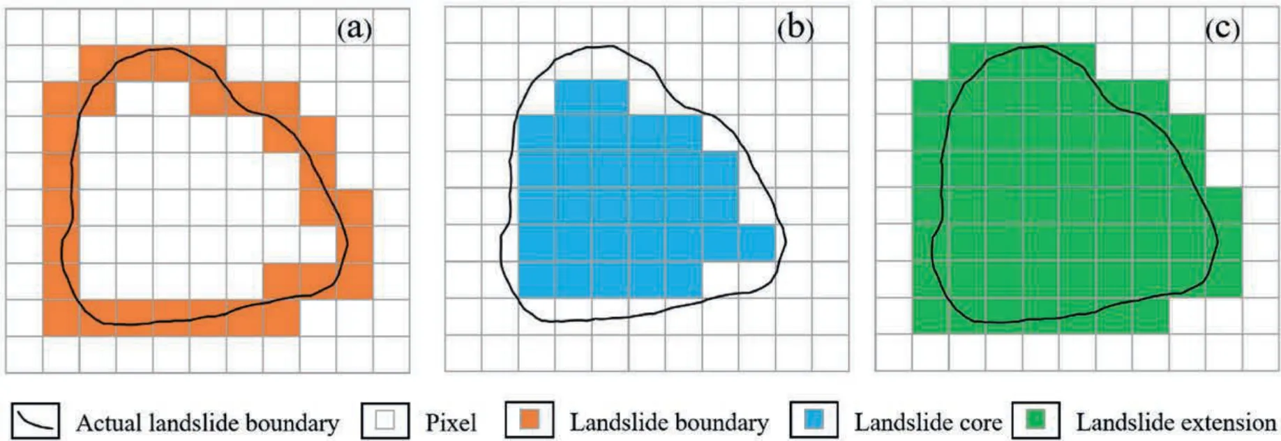
Fig.4.Different rasterization ways to represent a landslide with pixels: (a) Landslide boundary,(b) Landslide core,and (c) Landslide extension.
3.4.2.Non-landslide sampling strategy
Different from landslide samples,the sampling of non-landslide dataset is highly subjective.In literature,non-landslide samples were mostly randomly sampled from landslide-free area (Fig.5a),thus this strategy was selected as the reference scenario in the present study.Regarding the controlling test,non-landslides were sampled from the buffer zone and the very low(VL) susceptibility zone generated from some models.The buffer zone is obtained by taking the centre of any landslide point and drawing a circle surface with the buffer distance as the radius,then taking the intersection of the circle surface.The buffer zone scenarios included the buffer distance to landslides of<200 m(Figs.5b),200-400 m(Fig.5c)and outside of 400 m(Fig.5d),which were designed to reveal the effect of buffer distances on the sampling.
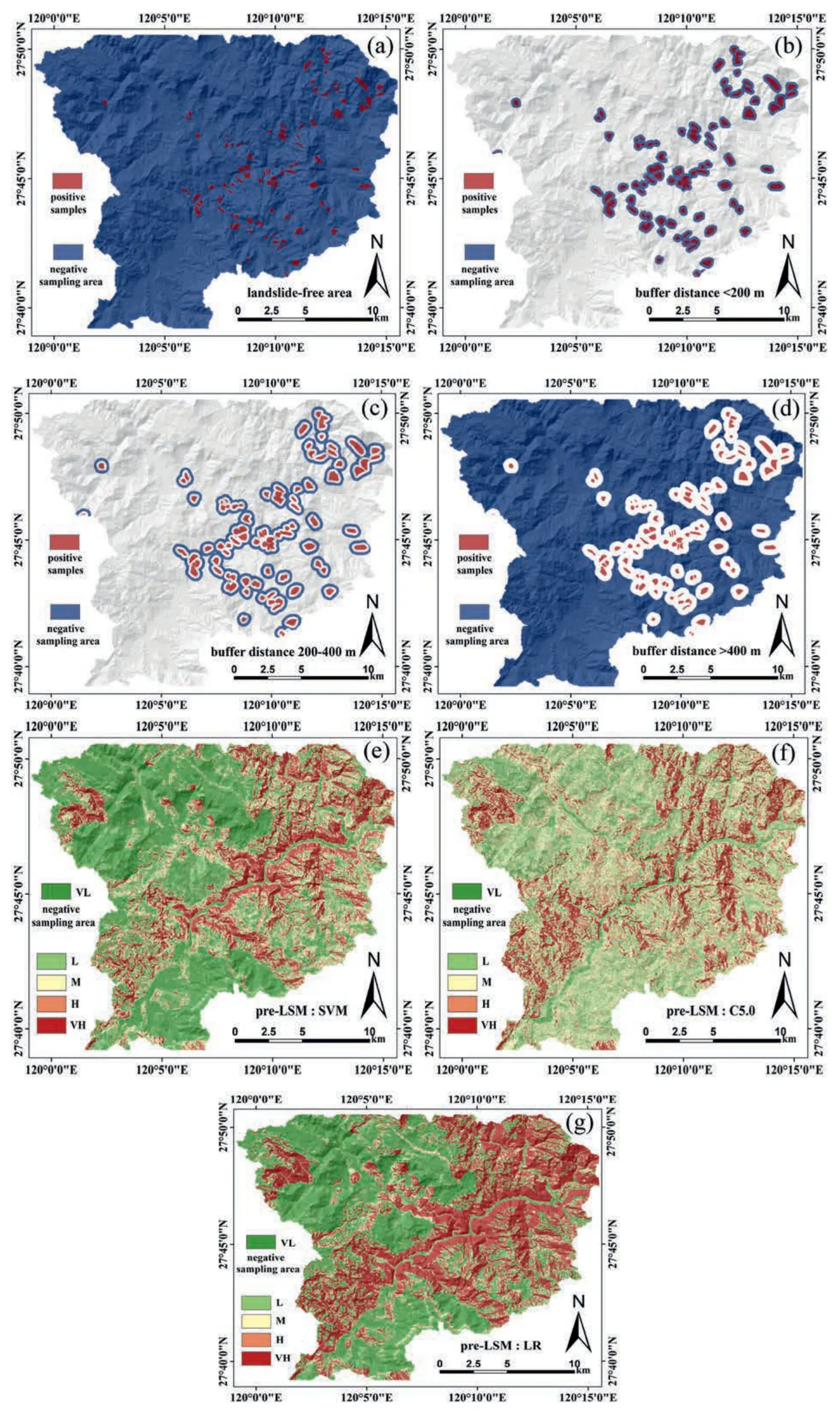
Fig.5.The negative sampling area for each sampling strategy:(a)Landslide-free area,(b)Buffer distance<200 m,(c)Buffer distance 200-400 m,(d)Buffer distance>400 m;(e),(f) and (g) are the VL zone of pre-LSMs generated by SVM,C5.0 and LR models,respectively.
Given that the LSA results mark different from model to model,two types of data-driven models,including generalized linear model (LR) and nonlinear regression model (C5.0 and SVM) were selected to generate landslide susceptibility maps in advance(pre-LSM) (Fig.5e,f,and g).Then the VL zones in these pre-LSMs were used to prepare for formal non-landslide datasets.It should be noted that the pre-LSMs were generated by using the non-landslide samples from landslide-free area and combined with equal landslide samples.
Finally,fourteen scenarios were determined by combining the landslide and non-landslide sampling methods mentioned above,and the specific information are shown in Table 2.An equal number of landslide and non-landslide samples were selected to ensure a balance of positive and negative samples in the modelling dataset in SPSS Statistics software.Then,the LSIs of the recorded landslide samples were set to 1,whereas those of the randomly selected nonlandslide samples were set to 0.As Shirzadi et al.(2017)suggested,the ratio of training to test datasets at 8:2 could obtain higher prediction accuracy in the raster resolution of 30 m.Thus,80% of the modelling datasets (composed of equal landslide and nonlandslide samples) under each scenario were randomly selected for the RF model training.The remaining 20%of the datasets were used for the test in SPSS modeler software.
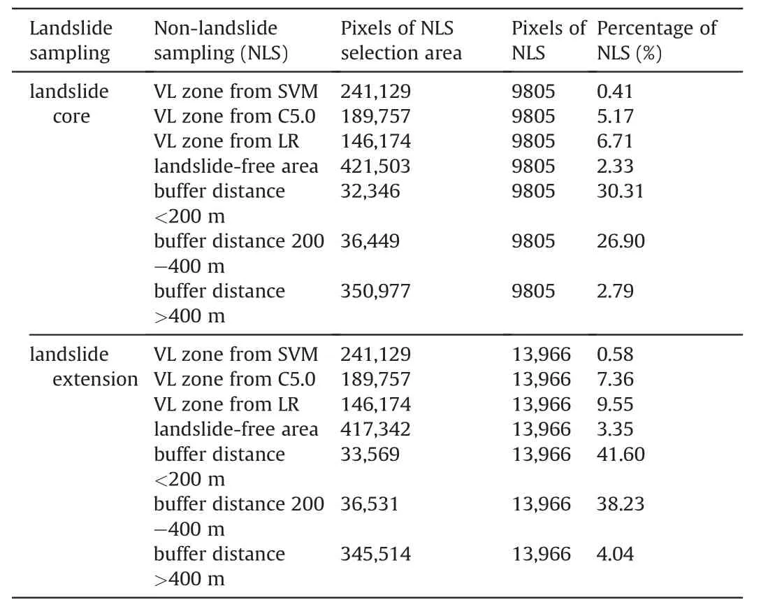
Table 2 The landslide and non-landslide sampling strategy of each scenario.
3.5.Contribution of influencing factors
The evaluation of the importance of the influencing factors can reflect the reasonableness of the links established between the model and the actual geological environment,and help to establish a system of influencing factors suitable for landslide susceptibility analysis (Liang et al.,2021).In this study,the importance of ten influencing factors was assigned by RF model in SPSS modeler 18.Then each of the importance indices was normalized using the max-min method,which was calculated as the following equation:
wherefiandfi* denote the values before and after normalization respectively,fminandfmaxare the minimum and maximum values in the data.
3.6.Model performance evaluation
ROC curve is known to be used to evaluate the accuracy of binary classification tasks in machine learning models and is widely used in the analysis of LSA results(Rodrigues et al.,2021).The horizontal axis and vertical axis of the ROC curve are combined by 1-specificity and sensitivity,and the AUC of the ROC curve ranges from 0 to 1,closer to 1 indicates better model performance.
where the value ofrankiis the number of thei-th sample,MandNare the number of positive and negative samples,respectively.
4.Results
4.1.Factor importance and LSM
Based on the principles introduced before,the influencing factors were reclassified and the FR values of each category are shown in Table 3.We can see that the impacts of different factors and categories on the occurrence of landslides have evident differences.For instance,the FR values were all greater than 1 when the slope degrees larger than 37°,and increased with the increase of the degree.However,the FR values of the slope degrees lower than 37°were smaller than 1,thus indicating the negative effect on landslide occurrences in the study area.Regarding the soil factor,the FR values of all soil types were lower than 1 except the red soil,which indicated that this type of soil was the most important for the development of shallow landslides.This can be explained by the large porosity of red soil,thus its strength decreases more rapidly when exposed to water(Su et al.,2015).The classifications in land cover factor that had larger impacts on landslides included dryland(FR=1.93),shrubs (FR=1.09),open grass (FR=1.50) and urban land(FR=1.17).Regarding the distance to river,the overall trend is that the FR values decreased with the increase of distance rivers,which agreed well with the spatial distribution of landslides in the area.
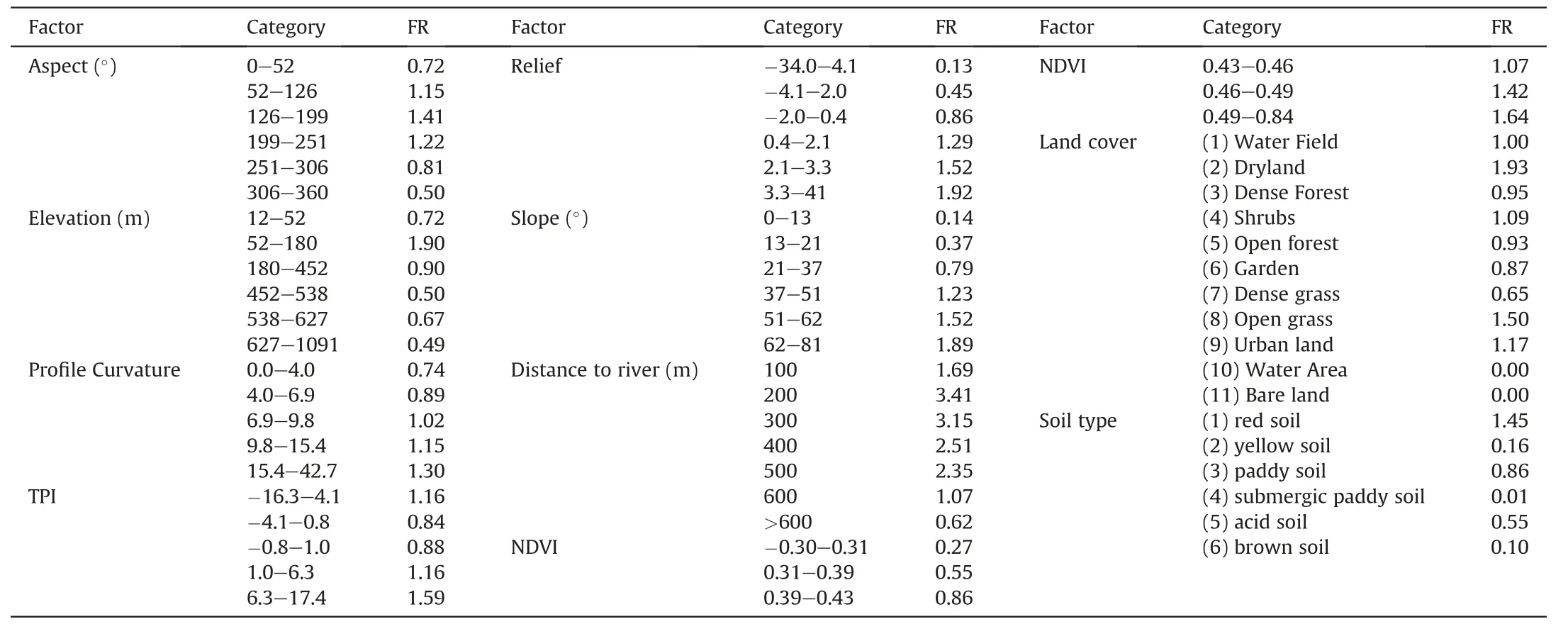
Table 3 The frequency ratio of each category within the influencing factors.
As seen in Fig.6,the importance of each influencing factor,which was represented by the importance measure(IM)value,was obtained from the RF model.We can see that six factors contributed more to the landslides in the study area,namely land cover(IM=1),soil type(IM=0.949),slope(IM=0.923),distance to river(IM=0.846),NDVI(IM=0.769),elevation(IM=0.641).The other four factors had relatively lower importance and their IM values were below 0.5.In general,the current results showed that the development of shallow landslides in the region was mainly controlled by the material (soil type),shape (slope),and surface covers(land cover,NDVI)of slopes.Moreover,no importance of the factors was smaller than 0,thus indicating it is reasonable to include these factors into the LSA of the study area.
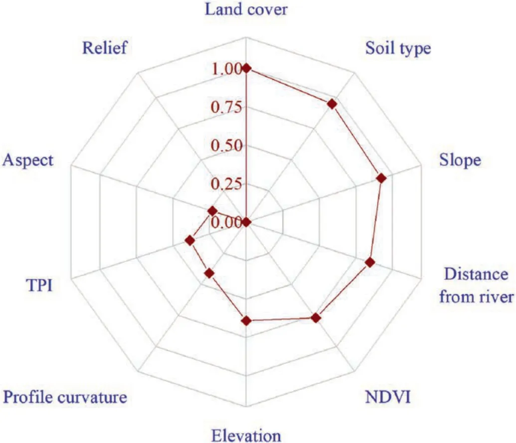
Fig.6.Radar chart of the importance of the influencing factors,in which the numbers show the IM value of each factor obtained from the RF model.
Fourteen final LSMs were generated for different scenarios based on the RF model.The whole area was divided into five zones based on the natural breaks method,namely very-low susceptibility(VL),low susceptibility(L),moderate susceptibility(M),high susceptibility (H),and very high susceptibility (VH),as shown in Figs.7 and 8.On the whole,although the LSMs under different scenarios are different,the distribution of VH,VL zones has similar patterns.The VH zones are mainly distributed at the river banks,since most settlements are located in this region,and human engineering activities can easily change slope stability.Another obvious VH zone is located in the mountainous area of the northeast which is characterized as higher altitude and larger relief.TheVL area is mainly located in the central and northwestern part with relatively gentle terrain.Although the susceptibility zonation varies with scenarios,all these maps can generally reflect the development trend of landslides in the region.Regarding the comparison among different sampling scenarios,the maps using landslide core(Fig.7) have more VH zone and less M zone than that using landslide extension dataset(Fig.8).Moreover,when the buffer distance applied for non-landslide dataset increases,the VL and VH zones become larger (Fig.7b-d,Fig.8b-d).

Fig.7.The landslide susceptibility maps generated by using the landslide core as positive samples,where the negative dataset was sampled from:(a)Landslide-free area,(b)Buffer distance <200 m,(c) Buffer distance 200-400 m,(d) Buffer distance >400 m;(e),(f) and (g) are the VL zone of pre-LSMs obtained from the SVM,C5.0 DT and LR models,respectively.
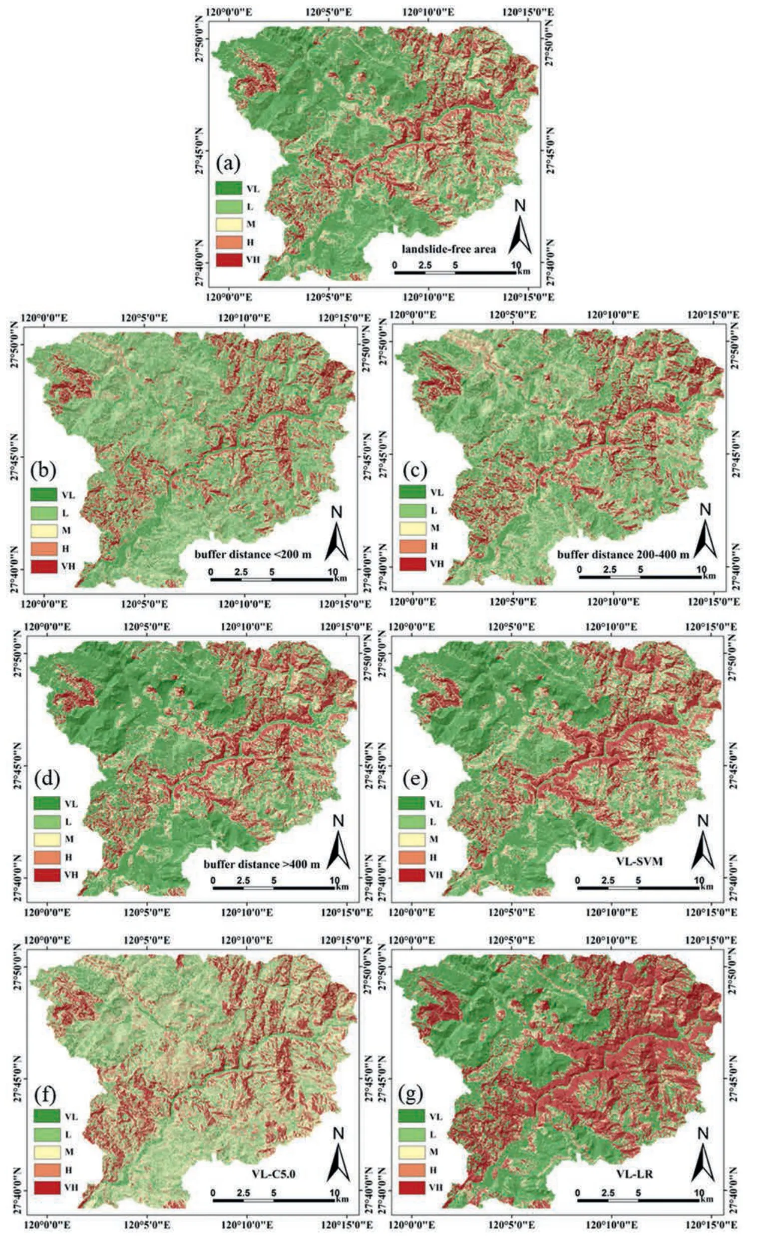
Fig.8.The landslide susceptibility maps generated by using the landslide extension as positive samples,where the negative dataset was sampled from:(a)Landslide-free area,(b)Buffer distance <200 m,(c) Buffer distance 200-400 m,(d) Buffer distance >400 m;(e),(f) and (g) are the VL zone of pre-LSMs obtained from the SVM,C5.0 DT and LR models,respectively.
4.2.Model performance evaluation and comparison
In order to reveal the distribution pattern of the susceptibility zonation and landslides in these LSMs,the area of each susceptibility level was first counted.The results show that the area of VH zone accounts for 12%-17% of the total area,and the area with medium susceptibility level accounts for 8%-30%.The area of L and VL zones are commonly larger than that of other susceptibility levels(Fig.9a and b).However,this is not the case when using the non-landslide dataset from the VL-LR model.In this scenario,the area of VH zone is rather large,which reaches 39% and 42%,respectively.Next,we compared the percentage of landslides in each susceptibility level.When the landslide core is utilized as positive samples(Fig.9c),the percentage of landslides identified in VL areas are no more than 2%,while this number can reach up to 90%in VH areas.In contrast,the landslide located in VL zone is less than 10%and the percentages of landslide in VH zones are between 44% and 83% when considering landslide extension as landslide dataset (Fig.9d).Then,the indicator of frequency ratio (FR) was calculated to represent the relatively density degree of landslides in a specific susceptibility zone which considered both landslide numbers and total area.Generally speaking,a reasonable landslide susceptibility map is characterized as higher FR values in high and very high susceptibility areas.In this study,the FR values for all scenarios increase with the increase of susceptibility level (Fig.9e and f).The FR values are less than 1 in low and very low susceptibility areas while larger than 1 in high and very high areas,thus indicating the landslide susceptibility zonation accurately captures the spatial distribution of historical landslides.It should be mentioned that the results regarding the scenario of VL-LR model is still an exception,where the FR values in H zone is less than 1,and FR in VH zones is evidently smaller than that in the other scenarios.This indicates that the performance by using the VL area from LR model as non-landslide dataset is not satisfactory.

Fig.9.The statistical indicators for the distribution of landslide susceptibility level and historical landslides: (a)The percentage of area of each landslide susceptibility level when using the landslide core dataset,(b) The percentage of area of each landslide susceptibility level when using the landslide extension dataset,(c) The percentage of landslides identified in each landslide susceptibility level when using the landslide core dataset,(d)The percentage of landslides identified in each landslide susceptibility level when using the landslide extension dataset,(e)The frequency ratio of historical landslides in each landslide susceptibility level when using the landslide core dataset,and(f)The frequency ratio of historical landslides in each landslide susceptibility level when using the landslide extension dataset.
Finally,the AUC values of training and testing datasets under 14 scenarios were calculated in SPSS modeler software to compare the performance of different sampling strategies (Fig.10).The AUC values range from 0.733 to 0.942,thus indicating that all the scenarios have good predictive results.Moreover,the results obtained by using the training dataset and test dataset have similar accuracies,which verifies the generalization ability of the applied methods.Among all the scenarios,the peak accuracy is from the result by using landslide core and VL-C5.0 model with the AUC value of 0.933(training dataset) and 0.942(testing dataset).
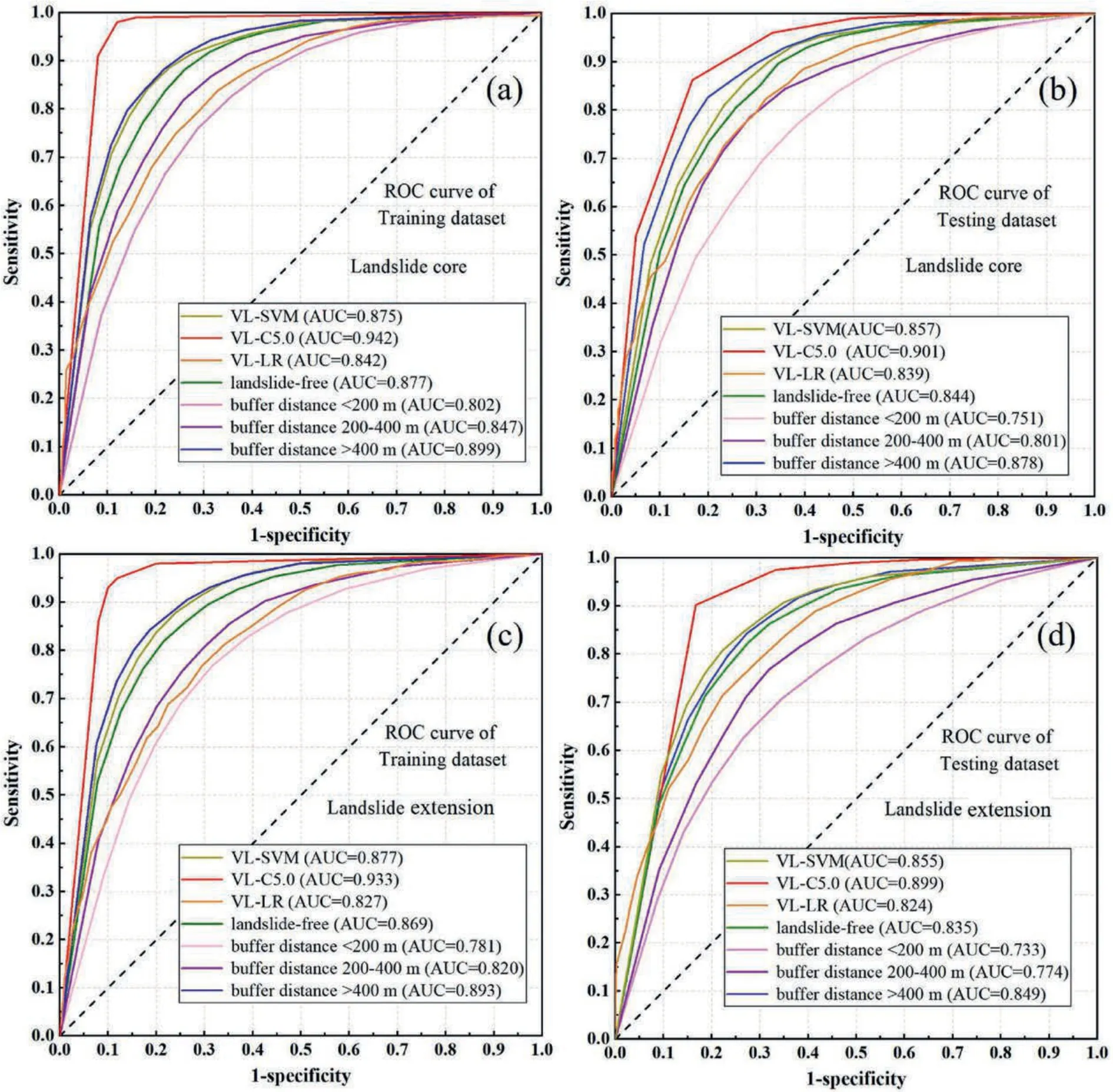
Fig.10.The ROC curves and AUC values of different scenarios.: (a) Using landslide core and training dataset,(b) Using landslide core and testing dataset,(c) Using landslide extension and training dataset,and (d) Using landslide extension and testing dataset.
4.3.Impact of sampling strategies on LSA
4.3.1.Impact of landslides sampling strategies
By comparing the landslide susceptibility maps of different scenarios,it can be found that the total area of H and VH zones of the maps applying landslide core as positive samples are slightly larger than those using the landslide extension dataset.Meanwhile,less L and VL zones are identified in the former maps than the latter ones.Moreover,the AUC values of the maps using landslide core are larger than those using landslide extension samples.Specifically,the maps using landslide core samples are larger than those using landslide extension by 0.2%-2.7% in AUC accuracy.These interesting results indicate that landslide cores can better reflect landslide characteristics,and better distinguish between landslide and non-landslide samples.This is mainly because that the landslide extension covers landslide boundary areas,which is the overlap zone between landslide and non-landslide.Pixels in these areas will dilute the landslide features and reduce the quality of landslide samples.Hence,it is recommended that users employ only landslide core as positive samples and discard pixels covering landslide boundary during landslide susceptibility modelling.
4.3.2.Impact of non-landslides sampling strategies
Considering the comparison results mentioned in the section above,the following analysis regarding non-landslide samples focus on the scenarios based on landslide core.Non-landslide sampling from landslide-free area is the most commonly used non-landslide sampling strategy,so this scenario is used as a reference to measure the magnitudes of change of modelling accuracy user the other scenarios.When the non-landslide dataset is obtained from the buffer zone around landslide boundary,the AUC accuracies improve with the increase of buffer distance.However,compared with the reference (AUC=0.844),only the scenario when the buffer distance larger than 400mhas better performance(AUC=0.878).The scenarios with the buffer distance of 200 m(AUC=0.751)and 200-400 m(AUC=0.801)are evidently lower in accuracy.This makes us conclude that the quality of non-landslide samples can be improved only when sampling at the area with a sufficient distance to landslide boundary.This can be explained that the pixels near from the landslide boundary have some similar characteristics with positive samples (landslide pixels) while the characteristics of negative samples (non-landslide pixels) are weakened.Therefore,the non-landslides dataset for machine learning model training are not representative enough.
Next,we assess the impacts of scenarios which use the VL zone from pre-LSM as non-landslide samples.It can be found that this sampling strategy can improve the performance of LSA.The AUC values are 0.857 (VL-SVM),0.901 (VL-C5.0) and 0.839 (VL-LR),respectively.It should be mentioned that the performance of the scenario applying the VL-LR model is not superior to that of the reference,which supports the results from the statistics of landslide distribution.Under this scenario(Fig.8g),the total area of high and very high susceptibility areas that were identified is larger than 50%of the entire region,which doesn’t agree well with the actual situation.Similar results are not observed in the scenarios which determine the non-landslides through the VL-SVM and VL-C5.0 methods.From the perspective of model principles,the RF,SVM,and C5.0 models are nonlinear models,while the LR is a linear one.The former is commonly more complex than the latter since the classification criteria for linear classification are homogeneous.Hence,the scenarios using the VL-SVM and VL-C5.0 methods conduct two nonlinear classification (the second one is the final LSM by using the RF model),which cause higher model accuracies.From the perspective of sample quality,the very low susceptibility zones from the LR model only focus on a part of characteristics of non-landslide sample,which causes that the missing characteristics are identified as high and very high susceptibility zones in the LSM.This is also the reason why this scenario has larger VH and H susceptibility zones than the other scenarios.Overall,the negative dataset sampled from very low susceptibility zone determined by machine learning models can improve the performance of LSA compared with that from the landslide-free area,but it is recommended to select nonlinear models.Therefore,among all the scenarios in this study,the one applying landslide core (positive dataset) and VL zone from C5.0 model (negative dataset) has the highest accuracy.
5.Discussion
In this section three main points will be discussed: (i) the uncertainties associated with the modelling strategy and results,(ii)main limitations of the current method and findings,and (iii) the comparison with previous studies.
The uncertainties of this study are mainly related to one of the following aspects:(i)the relationship between data resolution and landslide size,(ii) determination of buffer distance between landslide area and landslide-free area,and (iii) selection of influencing factors for the LSA.The landslides in the study area are mostly small-scale in volume (<105m3),with the area ranging from 478 m2to 0.05 km2.With the data resolution of 30m,landslide boundary commonly accounts for a large proportion of the entire landslide,which can result in a significant difference in the total area of landslide datasets between the two positive sample strategies.The statistical results confirm this point: the number of landslide pixels obtained from the landslide core is higher than those from the landslide extension by 40%.Hence,more fuzzy features related to the pixels covering landslide boundary are included into the positive dataset,leading to lower accuracies of the scenarios using landslide extension.It can be expected that the impact of sampling strategy of landslide dataset may decrease when it comes to large-scale landslides or higher resolution data.The choice of the proper resolution in LSM is always an operational issue,which is related to many aspects (Catani et al.,2013).Some studies test the performance of different data resolutions in regional LSM,but they failed to incorporate the variability of sampling strategy (e.g.Arnone et al.,2016;Schlögel et al.,2018).Hence,the future tests regarding the combined impacts of different scales,data resolution and sampling strategy may be of high interest.
Regarding the best definition of buffer distance for nonlandslide sampling,there is no agreement on this topic so far.In this study,a measurement in GIS shows that the average distance among the landslides in the study area is approximately 400m,thus we used the 200mas the interval for buffer distance but set only three scenarios(<200m,200-400m,>400m).There are also studies using 1 hm (e.g.Xi et al.,2022) or kilometer (e.g.Gameiro et al.,2021) as interval and defining more than 5 different buffer distances.Evidently,more intervals can more accurately capture the impact of buffer distance,but our current outputs reveal similar findings with the ones previously mentioned,namely the accuracy of LSM becomes higher with the increase of distance between landslide and non-landslide samples.Moreover,it should be noted that the definition standard of buffer distance in this study is different from previous ones.We separate the landslide free area into several individual parts without interactive overlap,instead of setting the area with larger distance than a certain threshold as an entire (Fig.11).Under this standard,we avoid potential repetitive sampling in landslide-free area.
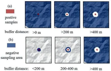
Fig.11.The comparison of buffer zone around landslide pixels: (a) Traditional buffer area used in the literature,and (b) The scenario used in this study.
The uncertainty originated from the influencing factors is dominantly associated with the model’s predictivity ability.Many environmental factors have been incorporated in landslide susceptibility modelling,but a “perfect” combination of factors does not exist (van Westen et al.,2006).In this study,we selected 10 factors,which agree with previous studies for similar test sites(e.g.Su et al.,2015),and each factor has been verified as reasonable through the calculation of importance(Fig.6).The results indicate that land use,slope,distance to river and NDVI are of higher importance for the landslide occurrence,thus partly supporting the point of Wang et al.(2020).However,there are studies revealing different findings where the important effect of rainfall on landslide susceptibility was emphasized (Su et al.,2015).In this study,the rainfall factor is discarded since it includes temporal information of landslides (Fell et al.,2008).Anyhow,the comparison regarding the factor importance makes us conclude that the contribution of factors may vary with local characteristics.Moreover,some studies show that eliminating or adding certain factors into a model may improve predictive ability (Pham et al.,2019;Tang et al.,2020),which was not conducted in this study because this is not our main objective.
Given the uncertainties mentioned above,the main limitations of the current method and findings can be summarized and stated.First,the influence of gridding methods of landslide samples on the model performance is greatly subject to the landslide area and type.However,limited by the type of slope failures in the study area,the current findings are only associated with shallow landslides.Second,the division of the buffer zone for the non-landslide samples is not detailed enough.Although the general law of the landslide susceptibility accuracy with the buffer distance was revealed,the optimal buffer distance has not been obtained.Finally,the results are not confirmed in other areas with different geological environments yet.Given that the accuracy of LSA is affected by many aspects,it is really difficult to directly predict the performance of the algorithm/model when it is applied for another region.We can only state that the performance of LSA is expected to be good when the proposed strategy is used for another similar area,when other procedures are normal.Therefore,it is necessary to verify the robustness and reliability of the obtained rules in other regions in future works.In spite of all these drawbacks,our results show that the uncertainty during the modelling process is acceptable: The AUC accuracy of all the scenarios is higher than 0.73 by using the testing dataset,and most scenarios have an accuracy larger than 0.8.This allows us to focus on the analysis of the impacts of sampling strategy instead of the improvement of model performance.
This study conducts an analysis of the combined impacts of landslide/non-landslide sampling strategy.It is difficult to directly compare our work to the other studies,because they often only considered one separate sampling strategy.For example,Dou et al.(2020) compared the performance of four different sampling techniques in LSM,and found that the order of predictive power is landslide scarp >landslide body >centroid of scarp >centroid of the body.Huang et al.(2022) tested the effects of different spatial shapes of landslide boundary,and confirmed better performance of landslide polygon in LSA.However,the investigation regarding the landslide expression was missing in the literature described above.Although the objectives are different,it seems that their works are useful supplementary for us,and a completed framework on landslide sampling strategy for different scenarios can be generated by combining current findings.Regarding the non-landslide sampling strategy,Lucchese et al.(2021) tested the performance by obtaining non-landslide samples from buffer zone and known lowlands,and found that a priori intervention on non-landslide samples (i.e.,sample from lowlands) can produce higher accuracy but are improper for generalization.This procedure needs rich expert knowledge to determine known non-susceptible area,but this is not available in the Feiyun catchment.Xi et al.(2022)compared the influences of the traditional buffer-controlled sampling method and a Newmark-based sampling approach for earthquake-triggered landslides,and found the latter one generated better results.Some other studies also have made attempts to obtain negative samples by machine learning models,including fractal theory(Hu et al.,2020)and self-organizing neural networks(Huang et al.,2017).Interestingly,their results all reveal that new strategies for sampling non-landslides can obtain higher predictive ability than traditional methods,which supports our results.Hence,it is necessary to develop and test more non-landslide sampling techniques as alternatives of traditional ones in the future,which would certainly provide new insights on this topic.
6.Conclusions
Regional LSA and associated uncertainties are one of the major challenges for landslide risk management and reduction.In the present study,the Feiyun catchment in southeast China was selected as a study area to test the impacts of sampling strategies of landslide and non-landslide datasets on the performance of LSM.Our results indicate that when the pixels covering only the landslide core are used as positive samples,the accuracy of LSM is higher than that of the map applying the pixels covering both landslide core and landslide boundary,with the improvement magnitude from 0.2% to 2.7%.A comparison regarding the nonlandslide sampling strategies showed that the negative samples from the very low susceptibility identified by nonlinear machine learning models can also improve the susceptibility modelling performance.Hence,the commonly used strategy which selects non-landslide samples from landslide-free areas may enlarge the uncertainty for the modelling.The results have demonstrated also that,the LSA can also have better performance when the nonlandslide dataset is determined from the buffer zone around landslide pixels.However,it should be noted that this improvement is closely related to the selection of buffer distance:when the buffer distance is less than 400 m,the accuracy of the landslide susceptibility map decreases instead.By combining different positive and negative sampling strategies,we determined 14 scenarios to generate regional landslide susceptibility maps.Among all the scenarios,the best predictive capability has been attributed to the landslide core(positive sample)and the very low susceptible zone from the C5.0 model (negative sample),with a peak AUC accuracy of 0.901.
Overall,the current test confirms that some uncertainties in LSA are associated with the dataset sampling strategy,but they can be reduced by improving the quality of positive and negative datasets.Hence,it is recommended to incorporate reasonable strategies regarding dataset sampling into the framework of LSM to make the outputs more reliable.Last,our future works can focus on the role of sampling strategy under different landslide sizes and data resolution.
Declaration of competing interest
The authors declare that they have no known competing financial interests or personal relationships that could have appeared to influence the work reported in this paper.
Acknowledgments
This research is funded by National Natural Science Foundation of China (Grant No 42307248) and Natural Science Foundation of Hebei Province (Grant No.D2022202005).Bixia Tian wants to thank the support from the Graduated Student Innovation Funding Project of Hebei Province (Grant No.CXZZSS2024007).
杂志排行
Journal of Rock Mechanics and Geotechnical Engineering的其它文章
- Using deep neural networks coupled with principal component analysis for ore production forecasting at open-pit mines
- Sliding behaviors of the trapezoidal roof rock block under a lateral dynamic disturbance
- Real-time arrival picking of rock microfracture signals based on convolutional-recurrent neural network and its engineering application
- Failure characterization of fully grouted rock bolts under triaxial testing
- Nonlinear constitutive models of rock structural plane and their applications
- Mechanical behaviors of backfill-rock composites:Physical shear test and back-analysis
