Using deep neural networks coupled with principal component analysis for ore production forecasting at open-pit mines
2024-03-25ChengkiFnZhngBeiJingWeiVictorLiu
Chengki Fn,N Zhng,Bei Jing,*,Wei Victor Liu,**
a Department of Civil and Environmental Engineering, University of Alberta, Edmonton, Alberta, T6G 2E3, Canada
b Department of Mathematical and Statistical Sciences, University of Alberta, Edmonton, Alberta, T6G 2G1, Canada
Keywords: Oil sands production Open-pit mining Deep learning Principal component analysis (PCA) Artificial neural network Mining engineering
ABSTRACT Ore production is usually affected by multiple influencing inputs at open-pit mines.Nevertheless,the complex nonlinear relationships between these inputs and ore production remain unclear.This becomes even more challenging when training data (e.g.truck haulage information and weather conditions) are massive.In machine learning (ML) algorithms,deep neural network (DNN) is a superior method for processing nonlinear and massive data by adjusting the amount of neurons and hidden layers.This study adopted DNN to forecast ore production using truck haulage information and weather conditions at open-pit mines as training data.Before the prediction models were built,principal component analysis(PCA)was employed to reduce the data dimensionality and eliminate the multicollinearity among highly correlated input variables.To verify the superiority of DNN,three ANNs containing only one hidden layer and six traditional ML models were established as benchmark models.The DNN model with multiple hidden layers performed better than the ANN models with a single hidden layer.The DNN model outperformed the extensively applied benchmark models in predicting ore production.This can provide engineers and researchers with an accurate method to forecast ore production,which helps make sound budgetary decisions and mine planning at open-pit mines.
1.Introduction
Oil sands mining is a vital pillar of Canada’s national economy(Stringham,2012).By 2035,it will provide more than 905,000 jobs and contribute $2.1 trillion to federal revenues (Honarvar et al.,2011).In oil sands mining,off-the-highway truck haulage is the predominant way for ore (e.g.oil sands) transportation from loading sites to dumping sites (Ma et al.,2021).Ore production by truck haulage (the total amount of ores transported by trucks) is directly associated with the overall production of mines(Baek and Choi,2020).Accurate forecasting of ore production by truck haulage will facilitate better mine planning (e.g.optimizing the fleet size and truck-shovel scheduling) and reasonable budgetary decisions for mining companies (Fan et al.,2023a).
In order to forecast ore production at mine sites,many scholars proposed simulation models and algorithms to calculate the amount of ores that can be hauled based on the sequential operations of trucks(Baek and Choi,2019;Fan et al.,2023b).For example,Jung et al.(2021) forecasted the ore production of underground limestone mines using a discrete-event simulation method.They proposed a simulation model based on various probability density distributions of truck travel times for the truck haulage system at mine sites.Other methods estimate ore production mainly by optimizing truck dispatchings or truck-shovel scheduling,such as linear programming (Benlaajili et al.,2020),integer programming(Mai et al.,2019),and stochastic optimization (Bakhtavar and Mahmoudi,2020).Nevertheless,these methods can be problematic due to unforeseen events at mine sites,such as work shifts,reduced equipment availability,and extreme weather conditions(e.g.rainfall and snowfall),thus affecting the prediction accuracy(Fan et al.,2023b).
To address the limitations in simulation methods,researchers have attempted to use historical datasets for constructing relationships(i.e.prediction models)between ore production and its influencing parameters (i.e.input variables) (Baek and Choi,2020;Choi et al.,2021;Jung and Choi,2021).These parameters include,but are not limited to,the number of dispatched trucks,time,speed,and distance-related variables at mine sites (Choi et al.,2021).For instance,Baek and Choi (2020) considered the number of trucks,the start and end time of truck haulage,the average wait time at dumping sites,and the average haul time to forecast ore production at an open-pit mine in South Korea.The same input variables were involved in estimating the ore production of a limestone mine in the research by Choi et al.(2021).The accuracy(e.g.the coefficient of determination,R2) of the prediction models in these studies attained 93%-98% (Choi et al.,2022).In addition,in our previous studies(Fan et al.,2022,2023a),input variables such as truck speed,haul distance,ambient temperature,and precipitation were adopted to forecast the productivity of truck haulage (a parameter directly relates to ore production),where theR2of the prediction models exceeded 86%.Each of these input variables played a crucial role in contributing to the model’s accuracy (Fan et al.,2023a).However,studies on prediction of ore production by incorporating truck haulage information and weather conditions are still scarce due to the high dimensional and nonlinear relationships between these numerous variables that need to be addressed.
Machine learning (ML) has garnered widespread attention in recent years for its capacity to establish complex relationships between numerous input and output variables(Farrell et al.,2019).ML is a collection of computational algorithms that model complex input-output relationships by automatically learning information from massive amounts of data (Fan et al.,2023a).ML usually includes deep neural network (DNN) and artificial neural networks(ANNs) (Oreshkin et al.,2021),support vector regression (SVR)(Khandelwal,2010),decision tree (DT) (Krzywinski and Altman,2017),random forest (RF) (Fan et al.,2023a),gradient boosting regression (GBR) (Friedman,2001),Gaussian process regression(GPR) (Zare Farjoudi and Alizadeh,2021),and k-nearest neighbors(KNN) (McRoberts,2012).Of these,DNN also belongs to deep learning,which is a more advanced concept based on traditional ANNs (Janiesch et al.,2021).DNN trains prediction models by adding multiple hidden layers (two or more) in the basic ANN structure (only one hidden layer) to achieve higher predictability(Baek and Choi,2020).For example,Li et al.(2022)constructed two prediction models(DNN and ANN)for detecting CO2concentration.The results presented that theR2of DNN (99.89%) with three hidden layers was greater than that of ANN (98.20%) with a single hidden layer.Moreover,the literature review shows that DNN usually outperforms the typical ML algorithms (Park and Park,2021).For example,Mahmoodzadeh et al.(2021) compared four typical ML models(SVR,DT,GPR,and KNN)with the DNN model for evaluating tunnel water inflow.The research showed that the prediction error (e.g.root mean square error,RMSE) of DNN was 4.67,whereas that of SVR,DT,GPR,and KNN was 12.96,17.99,5.77,and 16.64,respectively.Therefore,it is promising to apply DNN to build prediction models.However,according to the literature review,there is a lack of research on using the DNN algorithm to predict ore production by considering multiple input variables such as truck haulage information and weather conditions.
To this end,this study aimed to build a DNN model for forecasting ore production at open-pit mines using massive truck haulage information and weather conditions as training data.Unlike previous studies that directly built DNN models(Baek and Choi,2020),this study combined a dimensionality reduction technique(PCA)to preprocess massive data.PCA has been proven an efficient method to remove the multicollinearity between input variables and reduce the data dimensionality,thus making prediction models more reliable (Sulaiman et al.,2021).After that,DNN was used to handle numerous input variables and build complex nonlinear prediction models for ore production.Moreover,Bayesian regularized neural network (BRNN),back propagation neural network (BPNN),quantile regression neural network (QRNN),DT,RF,GBR,SVR,GPR,and KNN as benchmark models were built to be compared with the DNN model.
The novelty of this study resides in three points.First,unique data covering truck haulage information and weather conditions from open-pit mines were analyzed in depth.Second,this study adopted DNN for the first time to construct complex and nonlinear regression relationships by considering numerous input variables from truck haulage and local weather.Third,this study is the first one that combined PCA and DNN to deal with massive amounts of data and multicollinearity problems.The contribution of this paper is to build a DNN model based on PCA using truck haulage information and weather condition.This provides a more accurate method for mining companies to predict ore production,which helps make sound budgetary decisions and mine planning at openpit mines.
2.Methodology
2.1.Overview of the research framework
Fig.1 displays the research framework.The ore production data,containing truck haulage information and weather conditions,were split into training and testing subsets.Next,the variables in two datasets were scaled using a max-min normalization(normalized to between 0 and 1) (Arachchilage et al.,2023).After that,PCA was used to preprocess the input variables with strong correlations in the training dataset to reduce the data dimensionality.The resultant outcomes were applied to the testing dataset.Then,two types of neural networks were built based on the training dataset,including the proposed DNN with three hidden layers and the other three traditional ANNs (BPNN,BRNN,and QRNN) with only one hidden layer.In addition,eight commonly used ML models were constructed as benchmark models to be compared with the DNN model,including the DT,RF,GBR,linear kernel-based SVR(SVR (Linear)),polynomial kernel-based SVR (SVR (Poly)),radial basis function kernel-based SVR(SVR(RBF)),GPR,and KNN models.The hyperparameters established in these benchmark models were calibrated using a grid search approach based on five-fold crossvalidation,as this approach is easy to manipulate and has good optimization results (Erdogan Erten et al.,2021).Finally,three commonly used metrics were used to estimate the performance of the models: RMSE,MAE (mean absolute error),andR2(Wu et al.,2020).The whole training was conducted in RStudio with an R programming environment (version 4.1.3).
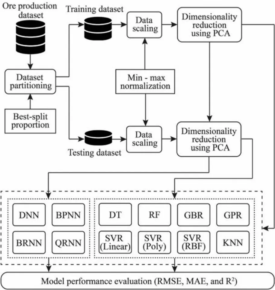
Fig.1.Overview of the research framework.
2.2.Machine learning algorithms
2.2.1.Single-hidden layer ANNs and multiple-hidden layer DNN
The commonly used ANNs that contain one hidden layer include BPNN (Oreshkin et al.,2021),BRNN (Goodarzi et al.,2010),and QRNN (Cannon,2011).They mainly differ in the settings of the weights and activation functions,resulting in models that exhibit different performances(Goodarzi et al.,2010;Wang and Syu,2016).However,unlike these traditional ANNs,DNN has more than one hidden layer,usually three or more,as shown in Fig.2b.This can add to the nonlinearity of the neural network,thus improving the generalization ability of prediction models (Li et al.,2022).To accurately predict the ore production,this study employed DNN with three hidden layers to build the prediction models and compared the performance with BPNN,BRNN,and QRNN with only one hidden layer.The basic principles of these neural networks are briefly described below.
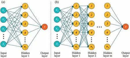
Fig.2.Schematic diagrams of the fundamental structures of (a) A standard artificial neural network and (b) A deep neural network.
In BPNN,input variables(i.e.neurons)are linked tonneurons of the hidden layer.The links are allocated weights (wij) that are linearly combined to produce the outputajof the hidden layer using an activation functionf(•)(Glória et al.,2016):
whereiindicates theith input neuron,jdenotes thejth hidden neuron,mis the number of input neurons,andbjrepresents a bias term.After that,the outputajis regarded as a new input with new weights (wij) connected to the output layer.Similarly,the sum of weights is converted to generate the output(y)of the output layer using an activation functiong(•)(Glória et al.,2016):
whereJis the number of neurons in the hidden layer,blis a bias term,lis the number of outputs.In order to reduce the prediction error,the weights and biases are updated by back-propagating the final output during the training process (Oreshkin et al.,2021).
BRNN is also an ANN that has only one hidden layer (MacKay,1992).The major difference between BPNN and BRNN lies in the choice of weights(Goodarzi et al.,2010).The former presumes that the weights are constant values,which may cause overfitting problems throughout the training process,while the latter treats the weights as arbitrary variables (Goodarzi et al.,2010).In BRNN,the weights (w) are assigned a prior probability distribution (e.g.Gaussian distribution),and then their posterior probability distributions are inferred based on Bayesian theory.
QRNN is another ANN algorithm with a single hidden layer structure proposed by Taylor (2000).It combines quantile regression and neural networks (Lu et al.,2022).Quantile regression approximates the model of the conditional median,which makes the minimum MAE value to estimate the conditional median of the target variable (Lu et al.,2022).When combined with neural networks,the weights in QRNN are transformed from the hidden to the output layers by applying the hyperbolic tangent to the inner product between the input and hidden layer weights.
DNN used in this study was constructed based on BPNN,as shown in Fig.2b.After processing in the multiple hidden layers,prediction results are derived through the path from the input layer to the output layer.The neurons in adjacent layers are concatenated by weights,and the sum of weights is also converted between the layers by an activation function.The widely used activation function in DNN is the rectified linear unit for regression problems(Baek and Choi,2020).In short,DNN increases the complexity of the prediction model by adding hidden layers and adjusting the neurons in each hidden layer,thus increasing the model’s nonlinearity and predictability.
2.2.2.Other ML algorithms
DT is a hierarchical-shape algorithm that contains a root node,internal nodes,leaf nodes,and branches between nodes (Breiman et al.,1984).RF and GBR are ensemble learning algorithms combining multiple DTs to perform better (Xue et al.,2020),as shown in Fig.3.RF uses a bagging technique to generate DTs,which includes two steps: bootstrapping and aggregation (Xue et al.,2020).“Bootstrapping” is a sampling method that trains each DT based on a randomly sampled subgroup (with replacement) from the original dataset.The final prediction is an average of the decisions made by all DTs,which is referred to as “aggregation”.Unlike RF,GBR adopts a boosting technique to generate DTs(Friedman,2001).In the boosting approach,there is learning,improvement,and correction of the prediction errors of the previous DT for each DT.This is different from the RF algorithm,where each DT is trained in an independent and parallel manner.

Fig.3.Schematic diagrams of the tree-based algorithms.
SVR is a supervised ML algorithm for regression tasks.In Fig.4,the space of input variables in SVR is split using optimum boundaries,also known as hyperplanes (Khandelwal,2010).SVR constructs the optimal hyperplane by maximizing the margin.Therefore,the vertical distance between the optimal hyperplane and the data points is minimized.These data points that are nearest to the margin are known as support vectors.When the data is indivisible in SVR,the high-dimensional space maps the data points(Boser et al.,1992).The mapping functions (i.e.,kernels),such as linear,polynomial,and radial basis functions,have been widely used in previous studies (Onyekwena et al.,2022).

Fig.4.Basic principle of support vector regression.
KNN is also a nonparametric technique that extracts information from the observed data to predict the output variables without defining a parametric input-output relationship(McRoberts,2012).In general,KNN achieves classification and regression in three steps:searching,calculating,and averaging.First,ksamples closest to a new data point are explored in the training dataset.After that,the separation of each sample from the new target data point is calculated.Finally,the outputs of theksamples are averaged as the output of the target new data point.
2.3.Principal component analysis
PCA is a practical and valuable statistical technique that transforms large correlated data into small uncorrelated data using principal components (PCs) (Shang et al.,2017).PCs can be expressed as linear combinations of the original input variables,which retain the complete information of the original data.To determine PCs,the eigenvalues λ (λ1≥λ2≥λ3≥…λm) and eigenvectorseof correlation matrix R can be obtained by
where I is the identity matrix.The eigenvalue indicates the amount of data variance that is interpreted by each PC (Cangelosi and Goriely,2007),which can be calculated by
According to the calculated variances,PC1 (the first one) corresponds to the linear combination of input variables and accounts for the maximum data variance.Next,PC2 (the second one) indicates the maximum variance,which is not accounted for by PC1.This process is repeated m times to obtain all PCs (PC3,PC4,…,PCm).In addition,the commonly used Kaiser rule was chosen to determine the number of PCs,which states that PCs with eigenvalues greater than one are reserved.In contrast,PCs with eigenvalues smaller than one do not deserve to be retained because they contain less information.(Coste et al.,2005).In this study,historical data at operating mine sites are observed with solid linear correlations among the input variables (explained in Section 3.1 in detail),leading to multicollinearity problems and decreasing the reliability of prediction models(Chan et al.,2022).PCA can control multicollinearity by analyzing the behavioral properties between variables,thus potentially improving model predictability (Baggie et al.,2018;Sulaiman et al.,2021).This provided the rationale for selecting PCA in this study.
2.4.Evaluation indexes
Correction indexes (i.e.performance metrics) are usually utilized to assess the model performance.These indexes are adopted to determine how well a prediction model can predict output variables on an unseen dataset.For regression tasks,the commonly used indexes include,but are not limited to,RMSE,MAE,andR2,which have been widely used in numerous application areas of mining engineering,such as rock strength (Hu et al.,2022),resource exploitation (Radwan et al.,2022),ground settlement(Tang and Na,2021),and cement material (Arachchilage et al.,2023).These three indexes are listed below(Huo et al.,2021):
where RMSE is the standard deviation of the residuals,MAE is the mean of the absolute errors,ynis the measured ore production,is the forecasted ore production,is the measured ore production mean.This study selected these indexes mainly because they can easily and quantitatively calculate the absolute or relative errors(residuals) between the measured and forecasted values,which displays an intuitive evaluation of model performance (Huo et al.,2021).Among these indexes,In general,the models that have a higherR2and lower MAE and RMSE perform better in prediction.
3.Data description and scaling
3.1.Data description
In this study,the dataset was collected from major production areas of oil sands in Alberta,Canada.It was derived from two main categories: truck haulage information and weather conditions,which reflected the hourly ore production of the oil sands mines for an entire year.The dataset contained a total of 8682 data points and was separated into a training subset (80%) and a testing subset(20%).This ratio was determined by investigating the effect of split proportions on PCA results and the model’s prediction accuracy,which will be discussed in detail in Section 4.1.The training dataset had 18 input variables and ore production (y,tonne);the testing dataset contained only 18 input variables because the testing dataset was used as a validation dataset.These 18 input variables were haul distance(x1,km),empty distance(x2,km),haul time(x3,min),empty time (x4,min),dump time (x5,min),wait time at shovel (x6,min),wait time at dump (x7,min),spot time (x8,min),haul speed (x9,km/h),empty speed (x10,km/h),number of trucks(x11),number of shovels(x12),ambient temperature(x13,°C),snow depth (x14,cm),month (x15),shift ID (x16),wind power (x17),and rainfall (x18).They were chosen mainly because of practicing engineers’experience and data availability at mine sites.Furthermore,distance,time,and speed-related variables of truck cycles have been considered influential parameters affecting ore production in previous studies (Choi et al.,2021).Moreover,hourly weather conditions (e.g.hourly ambient temperature)have been proven to be associated with the productivity of truck haulage,thus affecting ore production (Fan et al.,2023a).It is noted that the current dataset only involves hourly weather conditions.This is because the hourly data contain more data points(8682)and richer real-world information at mine sites than other time intervals (e.g.a daily dataset has up to 366 data points in an entire year).
Detailed information on the input variables is presented in Table 1.The first 14 inputs were numerical (or continuous),while the last four inputs were categorical.This represents the first 14 input variables had numerical values,while each categorical variable was composed of several labels.For example,the wind power and rainfall data were obtained from the local weather observatory(MEP,2019).According to the Beaufort Wind Scale (Wheeler and Wilkinson,2004),the wind power (i.e.,wind speed in our dataset) can be classified into six labels: (1) calm (0-1 km/h),(2)light air (1-5 km/h),(3) light breeze (6-11 km/h),(4) gentle breeze(12-19 km/h),(5) moderate breeze (20-28 km/h),and (6) fresh breeze(29-38 km/h).Similarly,according to the Manual of Surface Weather Observation Standards(MANOBS,2021),the rainfall in our dataset can be classified into three labels:(1)light rain(<2.5 mm/h),(2) moderate rain (2.6-7.5 mm/h),and (3) heavy rain(7.6-50 mm/h).In addition,the linear correlation was determined between every two variables by means of the commonly used Pearson correlation coefficient (r) (Baek and Choi,2020):

Table 1 A detailed description of 18 input variables (xi).
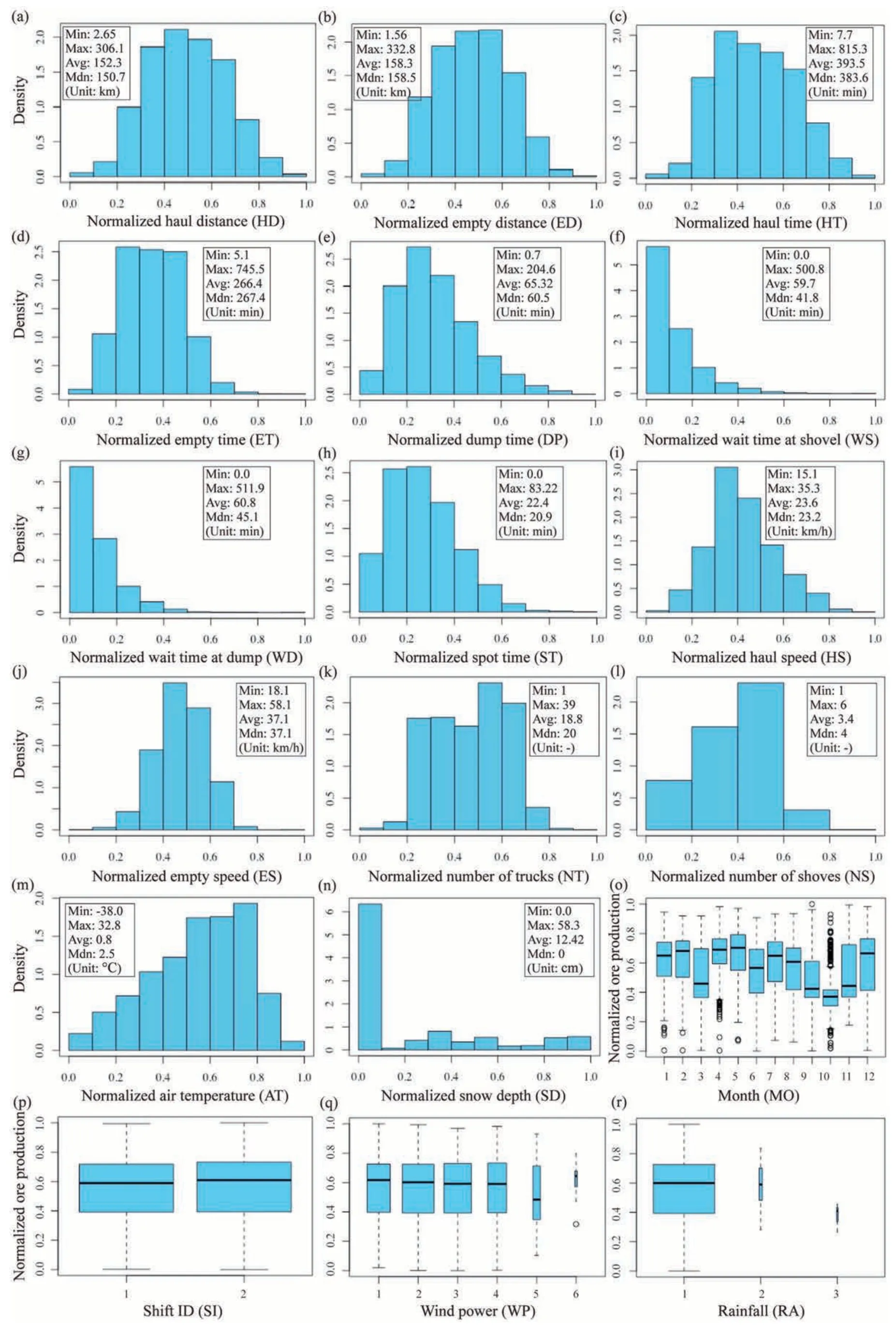
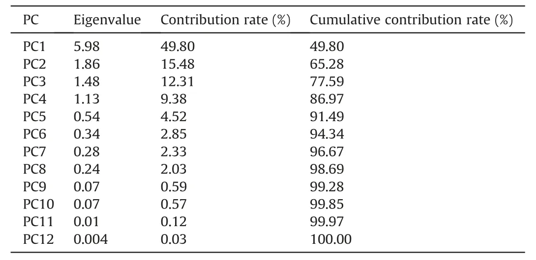
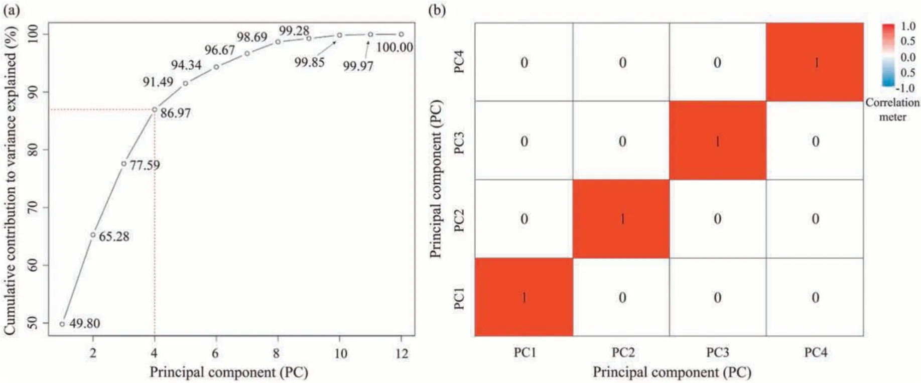
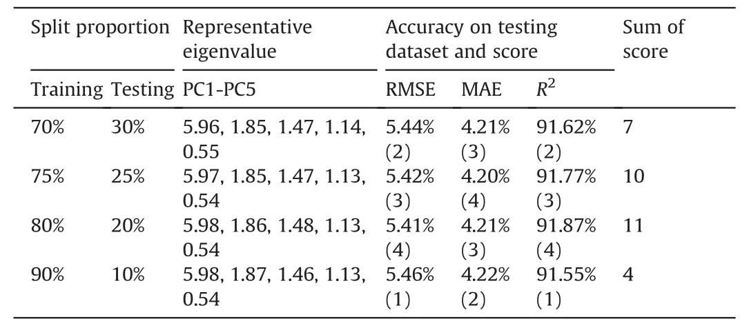
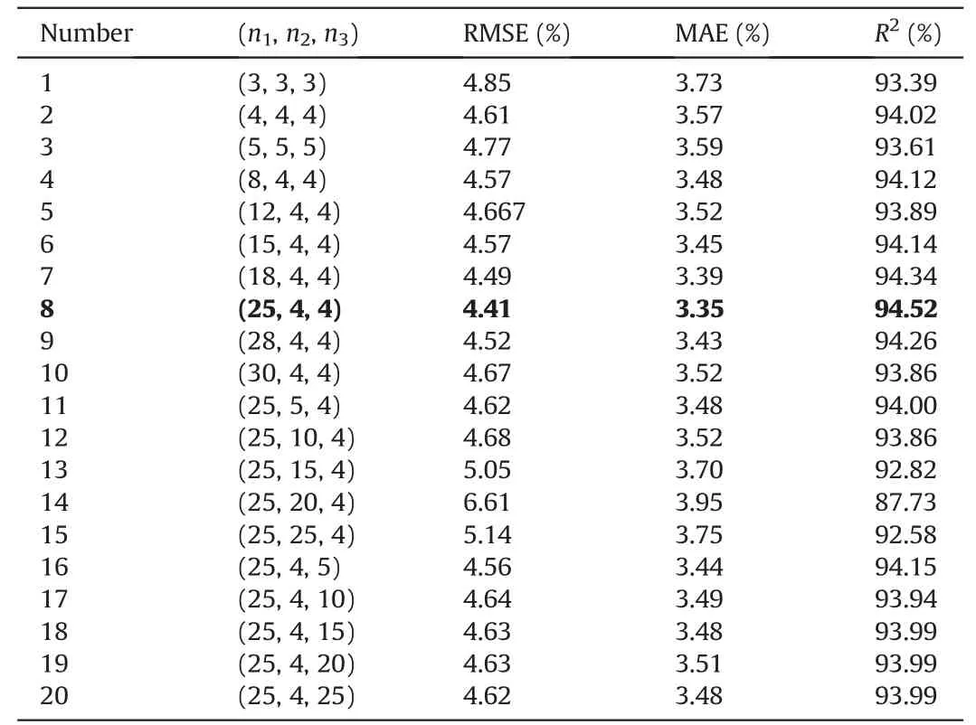
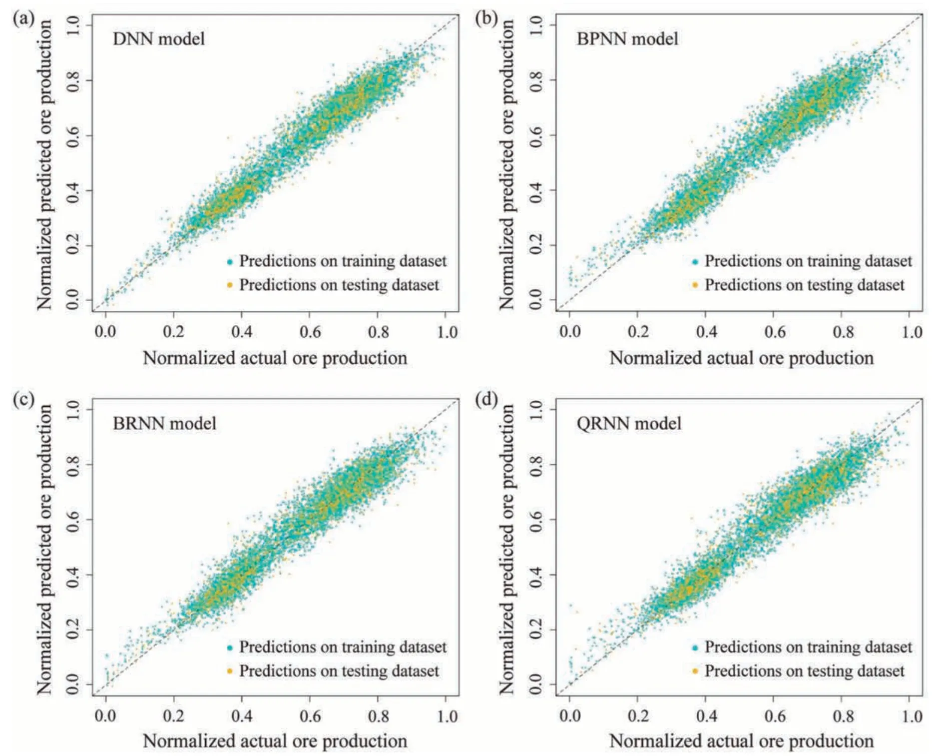
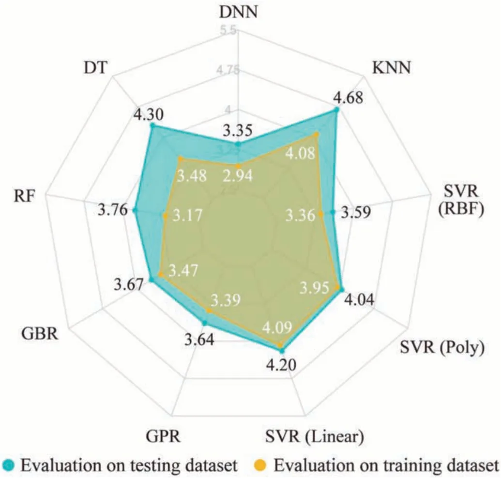
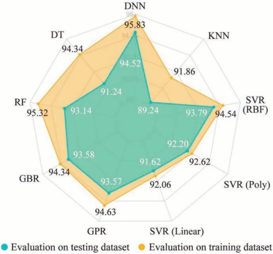
wherexmis themth input,is the mean of thexm,xnis thenth input variable,andis the mean of thexn.Table 2 lists therbetween these input variables.According to Ratner (2009),when 0.7 Banishing90 care, Prince Almas walked on through the garden, when suddenly a window opened and a girl, who was lovely enough to make the moon writhe91 with jealousy92, put out her head Table 2 Correlation coefficients (r) between the input variables. In this study,the input variables were measured at different scales.For instance,the range of the haul distance was between 2.7 km and 306.1 km,whereas that of the number of shovels was between 1 and 6.As a result,the statistical distributions of these variables varied significantly in their ranges,which may lead to some particular values (e.g.those in the upper range) playing a more critical role in model training,thus affecting the model accuracy (Arachchilage et al.,2023).Data scaling is a vital step in processing data because it can ensure that all variables are equal in relevance before building ML models (Ozsahin et al.,2022).Therefore,this study adopted commonly used min-max data scaling to normalize the statistical distribution of each variable(Arachchilage et al.,2023).Each continuous variable with numerical values was readjusted to be on the scale of zero to one using Eq.(10): wherex′means the normalized value,xrefers to the actual value,xminindicates the minimum of the x-variable,andxmaxis the maximum of thex-variable.Fig.5 presents the statistical distributions for all 14 inputs in the training dataset after data scaling. Fig.5.Distribution and statistics of inputs(Min:minimum,Max:maximum,Avg:average,and Mdn:median):(a)-(n)The histograms of 14 continuous input variables and(o)-(r)The boxplots for categorical inputs. In this study,the input variables with strong correlations were analyzed by PCA to reduce the dimensionality and multicollinearity in the training dataset.These input variables were haul distance(x1,km),empty distance (x2,km),haul time (x3,min),empty time (x4,min),dump time(x5,min),wait time at shovel(x6,min),wait time at dump(x7,min),spot time(x8,min),haul speed(x9,km/h),empty speed (x10,km/h),number of trucks (x11),and number of shovels(x12).These data were then fed into PCA to construct PCs,as shown in Table 3.Each PC has an eigenvalue that indicates the amount of variance being interpreted in the data (Cangelosi and Goriely,2007).The contribution rate is the percentage of variance interpreted by each PC;the cumulative rate of contribution is the cumulative percentage of variance interpreted from the first PC to the last PC (Holland,2008).According to Kaiser’s rule (Coste et al.,2005),PCs with eigenvalues larger than one are maintained,while PCs with eigenvalues smaller than one are not worth keeping because they contain less information.Therefore,the first four PCs(PC1,PC2,PC3,and PC4) were retained in this study,which explained 86.97% of the total variance,as shown in Fig.6a.Moreover,the correlation between these PCs was zero (Fig.6b),indicating that the multicollinearity was removed.This study is analogous to that of Li et al.(2015),who employed PCA to construct four PCs from four environmental input variables before establishing prediction models of the building’s electricity consumption.Through PCA,the first two PCs that interpreted 82.39% of the overall variance were kept,thus reducing the dimensionality of the original training dataset.In short,PCA eliminated redundant information in the data and identified essential input variables for building prediction models. Table 3 PCA results. Fig.6.Results of PCA and correlation analysis:(a)Scree plot:the cumulative contribution proportion of PCs;and(b)Heatmap:the correlation between the retained PCs,including PC1,PC2,PC3,and PC4. Furthermore,the effect of the split proportions of training and testing datasets on PCA results and model accuracy was investigated.The split proportions included 70%:30%,75%:25%,80%:20%,and 90%:10%,which are four proportions extensively applied in previous studies(Hou et al.,2022;Arachchilage et al.,2023).Table 4 lists the PCA results and the prediction accuracy of multiple linear regression(MLR)models based on four split proportions.MLR was adopted because of its ease of implementation,low computational effort,and less susceptibility to overfitting(Fan et al.,2022).As can be seen from Table 4,representative eigenvalues (PC1-PC5) of all four PCA results show that only the first four eigenvalues are larger than one.Therefore,PC1,PC2,PC3,and PC4 were preserved in each PCA with different split proportions.This indicates that the PCA results were not affected by the split proportions.In addition,Table 4 lists the performance comparison of the MLR models built based on four training datasets.The accuracy of each model was evaluated by three metrics and scored for each metric (ranging from one to four).The larger the RMSE and MAE,the low the score;conversely,the higher theR2,the greater the score.When the split proportion was 80%:20%,the model had the maximum sum of scores,indicating its highest prediction accuracy.Kumar et al.(2020) conducted similar work to investigate the effect of split proportion on the prediction accuracy of diabetes mellitus.They built DNN models based on three training datasets with different ratios and demonstrated that 80%:20%was the best ratio,with the DNN model achieving the highest accuracy of 98.16%.As a result,80%:20% was selected as the best-split proportion and utilized to construct more complex prediction models in this study. Table 4 Effect of split proportion on PCA and model accuracy. To establish DNN models,the four PCs retained in Section 4.1 were combined with the remaining six input variables from theoriginal training dataset to create a new training dataset.The new training dataset involved ten input variables: PC1,PC2,PC3,PC4,shift ID (label),month (label),ambient temperature (°C),snow depth(cm),wind power(label),and rainfall(label).In this study,all the DNN models included three hidden layers for constructing complex and nonlinear relationships between multiple inputs(ten input variables) and a single output (ore production).As a result,the structure of DNN models can be expressed as 10-n1-n2-n3-1,wherenjdenotes the amount of hidden neurons within thejth hidden layer.In addition,the number of neurons in each hidden layer varied between 3 and 30.To determine the optimal combination of the number of neurons,Table 5 summarizes part of the DNN models with different neural structures and their prediction performance evaluated based on the testing dataset. Table 5 Part of the DNN models with different structures and their performance on the testing dataset. In Table 5,when the number of neurons increased in a parallel manner in each hidden layer,the DNN model showed the highest performance with the neural structureof10-4-4-4-1,where the RMSE,MAE,and R2 were 4.61%,3.57%,and 94.02%.After that,the number of neurons was tuned separately in different hidden layers to investigate the changes in the DNN models’ performance.From Table 5,when the number of neurons approached 25 alone in the first hidden layer,the RMSE value was reduced from 4.61%to 4.41%.However,when the number reached 30,it increased to 4.67%.Thus,the optimal number of neurons was 25 for the first hidden layer.Likewise,the optimal number of neurons was decided to be 4 and 4for the second and third hidden layers when the minimum RMSE(4.41%),MAE(3.35%),and maximum R2(94.52%)were attained.Hence,the final proposed DNN model’s structure was 10-25-4-4-1,which refers to Fig.7 for a graphical demonstration.Akin to the study by Ly et al.(2021),they proposed a three-hidden layers DNN model to estimate the compressive strength of rubber concrete.According to their research,the DNN model had the highest accuracy with the number of neurons in the three hidden layers of 16,14,and 3,respectively,whereR2reached 97.50%. Fig.7.Schematic diagrams of the fundamental structures of the best DNN model. Furthermore,this study investigated the influence of truck haulage-related inputs and weather-related inputs on the prediction accuracy of DNN models,as shown in Table 6.Table 6 presents three scenarios:(1)considering all input variables(four PCs and the remaining six inputs),(2)excluding weather-related inputs,and(3)excluding truck haulage-related inputs.It can be noted that the accuracy of the DNN model dropped when input variables were continuously excluded.For example,theR2of the DNN model reached 80.73% when only trucking-related inputs were involved,compared to 10.32%for the DNN model that included only weatherrelated inputs.This suggests that the truck haulage-related inputs played a more critical role in predicting ore production than the weather-related inputs.The same results were found in our previous study,where the contribution of haul distance (43.51%) was more significant than that of ambient temperature (12.71%).Despite this,the weather-related inputs contributed to the model to some extent (10.32%).Sun et al.(2018) also reported a 5.13%improvement in the accuracy of the prediction model after taking weather factors into account. In this study,hyperparameters in 11 benchmark models were adjusted by a grid search approach based on five-fold cross-validation to control the complexity of the models.These benchmark models were BPNN,BRNN,QRNN,DT,RF,GBR,SVR (with three kernels),GPR,and KNN.To evaluate the effect of using this approach,the prediction error (e.g.RMSE as a metric) of these prediction models was calculated for each combination of hyperparameters within a predetermined search range.Table 7 lists the determined optimal hyperparameters for these models.With these optimal values,the benchmark models can avoid the risk of overfitting,thus exhibiting better prediction performance (Moayedi et al.,2019).This is compatible with the study of Arachchilage et al.(2023),who established four prediction models (i.e.ANN,RF,GBR,and SVR models) to forecast the uniaxial compressive strength of alkali-activated slag-based cemented materials.Compared with the preliminary models,the RMSE values of the ANN,RF,SVR,and GBR models reduced by 9.29%,1.45%,39.24%,and 39.81% after tuning hyperparameters,indicating that the model performance was improved. Table 7 Determination of hyperparameters for the benchmark models based on five-fold cross-validation. 4.4.1.Comparison of DNN,BPNN,BRNN,and QRNN models In this study,the proposed three-hidden layers DNN model and three single-hidden layer ANN models were used to predict ore production.Fig.8 presents the scatter points of the normalized expected ore production (vertical) from these models and the normalized measured ore production (horizontal).The diagonal line is an ideal line,indicating that the forecasted and measured values are equal.The minor deviation between the forecasted and measured values,the more uniformly the scatters are distributed along the diagonal(Fan et al.,2022).As shown in Fig.8,the points generated by these four models based on the training and testing datasets are closely dispersed along both sides of the diagonal.This indicated that these four models performed well in predicting ore production.In addition,Table 8 lists the quantitative performance metrics of these four models verified using training and testing datasets.From Table 8,the RMSE,MAE,andR2were 4.41%,3.35%,and 94.52% for the DNN model based on the testing dataset.Accordingly,these indicators were 4.88%,3.74%,and 93.29%for the BPNN model,4.7%,3.6%,and 93.78%for the BRNN model,and 4.83%,3.65%,and 93.44%for the QRNN model.Regarding theR2alone,the predictability of these four models was ranked as DNN(94.52%)>BRNN(93.78%)>QRNN(93.44%)>BPNN(93.29%).The same finding was seen by Maldonado et al.(2020),who developed two models to predict complex traits for genomic selection using DNN and BRNN.The results demonstrated that the predictability of the DNN (0.78) model was higher than that of the BRNN (0.71)model.Similarly,Lu et al.(2022) and Oreshkin et al.(2021) both demonstrated that DNN models performed better than QRNN and BPNN models in electricity load forecasting.In summary,the proposed DNN model with multiple hidden layers outperformed the traditional ANN models (having a single hidden layer) when predicting ore production at open pit mine sites. Table 8 Performance of the DNN,BPNN,BRNN,and QRNN models on training and testing datasets. Fig.8.Scatterplots of the normalized actual ore production and normalized predicted ore production.The evaluation results from the (a) DNN model,(b) BPNN model,(c) BRNN model,and (d) QRNN model. 4.4.2.Comparison of DNN,DT,RF,GBR,SVR,GPR,and KNN models To further evaluate the DNN model’s prediction performance,six commonly applied ML algorithms were adopted to build eight additional benchmark models.These were the DT,RF,GBR,SVR(Linear),SVR (Poly),SVR (RBF),GPR,and KNN models.Figs.9-11 are three radar charts for illustrating the performance evaluation(using RMSE,MAE,andR2) of these eight benchmark models and the DNN model based on the testing and training datasets.In each chart,the vertices of the irregular polygons represent the nine models.The proximity of the vertices from the center along the axes is the performance measure for each model.For example,in Fig.9,regarding the testing dataset,SVR(RBF)had the lowest RMSE value (4.7%) among the benchmark models,indicating that it outperformed the other benchmark models.Despite this,the DNN(4.41%)model achieved a lower RMSE value compared with the SVR(RBF) (4.70%) model.Therefore,the DNN model performed better than these benchmark models.This applies to the evaluation metrics of MAE (Fig.10) andR2(Fig.11) in this study.The same finding was found by Park and Park(2021):the RMSE value of the DNN (226.73) model was lower than that of the SVR (380.63),RF(357.18),GBR(367.11),GPR(372.7),and KNN(363.45)models when predicting the natural ventilation rate of sustainable buildings.Olu-Ajayi et al.(2022) also reported that DNN (e.g.RMSE=1.16) outperformed other traditional ML models,such as BPNN (1.2),GPR(1.4),SVR (1.61),RF (1.69),KNN (2.4),and DT (2.55) in predicting building energy consumption. Fig.9.Performance of the DNN,DT,RF,GBR,GPR,SVR,and KNN models evaluated by RMSE (in percentage) based on training and testing datasets. Fig.10.Performance of the DNN,DT,RF,GBR,GPR,SVR,and KNN models evaluated by MAE (in percentage) based on training and testing datasets. Fig.11.Performance of the DNN,DT,RF,GBR,GPR,SVR,and KNN models evaluated by R2 (in percentage) based on training and testing datasets. Moreover,two additional findings can be concluded from comparing these benchmark models: (1) the SVR model with the RBF kernel performed better in predicting the ore production than the SVR model with the other two kernels (Linear and Poly).For instance,for the testing accuracy,theR2of the SVR (RBF) was 93.79%,while those of the SVR(Linear)and SVR(Poly)were 91.62%and 92.2%.Onyekwena et al.(2022) also proved that the performance (R2) of the SVR (RBF) (99.25%) model was higher than the SVR (Linear) (94.15%) and SVR (Poly) (92.06%) models when predicting gas diffusion coefficient of biochar-amended soil (2) the tree-based ensemble models (i.e.GBR and RF);performed better than the single DT model.For example,for the testing accuracy,the MAE value of the DT(4.3%)model was more significant than the RF(3.76%) and GBR (3.67%) models.This is consistent with our previous study of mine truck productivity using tree-based models(Fan et al.,2023a).In conclusion,the DNN model had the greatest predictability through comparative studies,which provides the resource industry with an accurate method to forecast ore production and help to make budgeting decisions and mine planning. In this study,the DNN model with a specific neural structure was proposed for forecasting ore production by truck haulage at open-pit mines.Unlike previous studies(Baek and Choi,2020;Choi et al.,2021,2022),this study combined truck haulage information from oil sands mines and local weather conditions as training data to construct a more accurate DNN model for predicting ore production at mine sites.For example,for the testing accuracy,theR2of the DNN model was 94.52%,which was higher than that of the BPNN (93.29%),BRNN (93.78%),QRNN (93.44%),DT (91.24%),RF(93.14%),GBR (93.58%),SVR (RBF) (93.79%),SVR (Linear) (91.62%),SVR (Poly) (92.20%),GPR (93.57%),and KNN (89.24%).In addition,this study preprocessed the input variables with strong correlation(r>0.7 orr<-0.7) using PCA before building the prediction models.The 12 input variables in the original dataset were reduced to four PCs by PCA.This effectively reduced the dimensionality of the training data to lower the computational complexity and resolved the multicollinearity between these input variables,making the proposed prediction model more reliable (Chan et al.,2022). Nevertheless,the proposed DNN model had its limitations.More future work is needed to improve the prediction model.First,other additional inputs that have not been considered may also influence ore production,such as tire properties (Ma et al.,2023),loaded speed (Fan et al.,2023a),pavement elevation (Chanda and Gardiner,2010),and driver habits (Sun et al.,2018).For example,Ma et al.(2021) reported that high tire temperatures could cause rubber failure of the off-the-road tire at mine sites,thus affecting the productivity of truck haulage and ore production.These potential influencing inputs may be added to future work to construct ore production prediction models at open-pit mines.Second,there are many more advanced methods for data dimensionality reduction,such as uniform manifold approximation and projection(UMAP),kernel PCA,autoencoders,and t-distributed stochastic neighbor embedding (t-SNE) (Gisbrecht et al.,2015;Sidhu et al.,2012).These advanced techniques may be more effective than PCA when the data are high-dimensional and present complex nonlinear relationships between variables (Anowar et al.,2021).Therefore,more comparative studies between methods are necessary for efficient dimensionality reduction.Third,the proposed model can forecast the hourly ore production by responding to the hourly weather conditions.However,the proposed model has limitations in responding to other temporal characteristics of weather conditions (e.g.daily,weekly,and monthly rainfall).The impact of different temporal characteristics may vary on model prediction accuracy (Wen et al.,2019).For instance,the effect of daily rainfall on ore production may be greater than the hourly rainfall because of road conditions.Therefore,more investigations relating to temporal effects will be conducted in future work.Finally,this study utilized a grid search approach to tuning the hyperparameters,but grid search is not the only optimization method.Other algorithms have been proven helpful in tuning hyperparameters,such as genetic optimization (Chung and Shin,2020),whale optimization (Nguyen et al.,2021),and particle swarm optimization (Bardhan et al.,2022) algorithms.Therefore,these optimization algorithms will be utilized in future work to enhance the generalizability of the prediction model. Deep neural network(DNN)is suitable for processing nonlinear and massive data,which increases the model complexity and nonlinearity by adjusting the number of neurons and hidden layers,thereby adapting to the growing data size and improving the model predictability (or generalization).This work was the first studyincorporating truck haulage information and weather conditions as training data to construct a principal component analysis (PCA)-based DNN model for forecasting ore production at open-pit mines.Additionally,11 benchmark models were established to be compared with the DNN model to assess its performance.From this study,the main findings are listed as follows: (1) The DNN model with multiple hidden layers (i.e.three hidden layers)outperformed the ANN models with only a single hidden layer.For example,In terms ofR2alone,the predictability of the DNN model with three-hidden layer(94.52%) was higher than that of the BPNN (93.29%),BRNN(93.78%),and QRNN (93.44%) models,which contained only one hidden layer. (2) The DNN model performed better than the commonly used machine learning models(benchmark models)in predicting ore production.For instance,in terms of the testing dataset,radial basis function kernel-based support vector regression(SVR (RBF)) had the lowest RMSE value (4.7%) among the benchmark models,indicating that it outperformed the other benchmark models.Despite this,the DNN (4.41%)model achieved a lower RMSE value compared with the SVR(RBF) (4.7%) model. (3) The truck haulage-related inputs played a more critical role in predicting ore production than the weather-related inputs.For example,theR2of the DNN model reached 80.73%when only trucking-related inputs were involved,compared to 10.32% for the DNN model that included only weatherrelated inputs. (4) The predictability of the SVR(RBF)model was better than the linear kernel-based SVR model (SVR (Linear)) and the polynomial kernel-based SVR model (SVR (Poly)).For instance,for the testing dataset,theR2of the SVR (RBF) was 93.79%,while those of the SVR (Linear) and SVR (Poly) were 91.62%and 92.2%. (5) The tree-based ensemble models had higher accuracy than the single decision tree (DT) model.For example,for the testing dataset,the MAE value of the DT (4.3%) model was more significant than the random forest(3.76%)and gradient boosting regression(3.67%) models. (6) The DNN model with the neural structure of 10-25-4-4-1 was proposed for ore production forecasting due to its superior performance over the others.In this study,the DNN models achieved the highest accuracy,with anR2of 94.52%.This can provide mining companies with an accurate method to forecast ore production,which helps make sound budgeting decisions and mine planning. Declaration of competing interest The authors declare that they have no known competing financial interests or personal relationships that could have appeared to influence the work reported in this paper. Acknowledgments This work was supported by the Pilot Seed Grant (Grant No.RES0049944) and the Collaborative Research Project (Grant No.RES0043251) from the University of Alberta.
3.2.Data scaling
4.Results and discussion
4.1.Data preprocessing using principal component analysis
4.2.Development of deep neural network models

4.3.Determination of optimal hyperparameters

4.4.Performance of the proposed model


4.5.Advantages, limitations, and future work
5.Conclusions
杂志排行
Journal of Rock Mechanics and Geotechnical Engineering的其它文章
- Sliding behaviors of the trapezoidal roof rock block under a lateral dynamic disturbance
- Real-time arrival picking of rock microfracture signals based on convolutional-recurrent neural network and its engineering application
- Failure characterization of fully grouted rock bolts under triaxial testing
- Nonlinear constitutive models of rock structural plane and their applications
- Mechanical behaviors of backfill-rock composites:Physical shear test and back-analysis
- Slope stability of reclaimed coal mines through a new water filling index
