A Study on the Transmission Dynamics of the Omicron Variant of COVID-19 Using Nonlinear Mathematical Models

S.Dickson ,S.Padmasekaran ,Pushpendra Kumar ,Kottakkaran Sooppy Nisar and Hamidreza Marasi

1Department of Mathematics,Periyar University,Salem,Tamilnadu,636011,India

2Faculty of Engineering and Natural Sciences,Istanbul Okan University,Istanbul,Turkey

3Department of Mathematics,College of Science and Humanities in Alkharj,Prince Sattam Bin Abdulaziz University,Alkharj,11942,Saudi Arabia

4Department of Applied Mathematics,Faculty of Mathematics,Statistics and Computer Science,University of Tabriz,Tabriz,Iran

ABSTRACT This research examines the transmission dynamics of the Omicron variant of COVID-19 using SEIQIcRVW and SQIRV models,considering the delay in converting susceptible individuals into infected ones.The significant delays eventually resulted in the pandemic’s containment.To ensure the safety of the host population,this concept integrates quarantine and the COVID-19 vaccine.We investigate the stability of the proposed models.The fundamental reproduction number influences stability conditions.According to our findings,asymptomatic cases considerably impact the prevalence of Omicron infection in the community.The real data of the Omicron variant from Chennai,Tamil Nadu,India,is used to validate the outputs.

KEYWORDS Omicron;local stability;reproduction number;steady states;global stability

1 Introduction

Since COVID-19 is a newly discovered virus,little is known about how it spreads.As a result,health authorities must thoroughly understand the incubation and recovery periods to implement more efficient quarantine procedures for those suspected of carrying the virus.As of November 24,2021,Omicron has been found in countries,and it continues to be the most popular variant all over the world.The transmission dynamics and the potential roles of various intervention strategies have been better understood by recent COVID-19 studies[1–7].These methodologies incorporate relief and concealment to dial back the spread of the pandemic,decreasing pinnacle medical care to safeguard the people who are most in danger from contaminations,lessening the number of infective cases to a low level,implementing lockdown to a district of exceptionally infective cases,confining suspect cases at home,isolating those residing in a similar family at home.Some authors developed an Omicron variant model with variable population size[8–14].

After becoming infected,a strengthening of the immune system may cause a delay in entering the infectious stage,and a significant amount of delay may even result in the disease being stopped at the exposure level.As a result,the effect of time delay on studying the dynamics of disease spread is significant.In addition,the effect of quarantine on preventing disease spread and the transmission of infection from both the exposed and infected groups are taken into consideration.On the one hand,people who were exposed have the virus,but unlike an asymptomatic patient,they do not show any symptoms right away.There is a latency period before an exposed person becomes infected,and it can take up to 14 days for some people to become infected.By developing the integer model,the current study aims to investigate the effects of the latency period.Using the delay differential equations model,newly infected individuals are given some time before contracting the disease.

To prevent COVID-19 infection in the host population,some authors developed delay-type models.Liu et al.proposed a time delay model and utilised the methodology to analyse the COVID-19 pandemic in China[15].A new form of disease model based on a time delay dynamics was developed in[16].They fitted model parameters based on the total number of reported cases in Beijing and Wuhan,China.Using mathematical and statistical modelling,Sedighe et al.developed a model to determine the epidemic trend and forecast the number of patients hospitalised due to COVID-19 in Iran [17].The SEIQR COVID-19 propagation model with two delays was investigated by Fangfung et al.in[18].Their model took supply chain transmission and hierarchical quarantine rate into account.A modified SIR model which combines suitable delay parameters and generates a more reliable forecasts of COVID-19 real-time data was proposed in[19].Where the authors compared the predictions of the recently constructed SIR model to actual data collected from Germany,Italy,Kuwait,and Oman.Shidong et al.created a delay SEIR model based on the feedback linearization technique to manage the effects of COVID-19[20].The authors in[21]proposed a SIRDV model to investigate the impact of vaccination campaigns during the pandemic in Israel and Great Britain.In[22],the authors introduced a time delay model considering the migration of individuals from susceptible to infected class.The Omicron model can be mathematically modeled in a way that is reasonably accurate to the occurrences that have been observed when delay factors are included in the system of differential equations.

In this paper,two delay mathematical models are proposed.The work is significant,because it contains the mathematical modeling with a real-data of the Omicron variant from Chennai,Tamil Nadu,India.In the form of sections,the delayed SQIRV model is proposed and its stability is examined in Section 2.The delayed SEIQIcRVW model is proposed and steady-state solution existence is tested in Section 3.In order to confirm and strengthen our theoretical findings regarding Omicron B.1.1.529 SARS-Cov-2,computational simulations are carried out from the real data which is collected from Tamilnadu in Section 4.In Section 5,we summarise our findings.

2 Delayed SQIRV Mathematical Model

Here we define the delay-type version of the integer-order SQIRV model proposed in [23].The disease is considered to have an incubation time ofτ >0,because the virus moved from the susceptible phase to the incubation phase.The time between becoming susceptible to the virus and experiencing its symptoms is referred to as the incubation period.Based on the policy decisions made by the government,a set of parameters have been obtained to forecast the pandemic trend.Table 1 lists the non-negative parameters that are used in this model.

Table 1:Parameters and their descriptions

Considering the given aspects,the delay SQIRV mathematical model is derived as follows:

whereη21=η1+η2,η22=η1+η4+η8,η23=η1+η7+η10+η12,η24=η1+η5+η11,andη25=η1+η6

Subject to initial conditionsS(0)=S0,Q(0)=Q0,I(0)=I0,R(0)=,V(0)=V0.

As in the case of Omicron,a susceptible individual is assumed to interact with an infected individual in the equation system but does not enter the infected compartment until after a predetermined incubation period.The incubation periodτis just while moving from the powerless compartment to the contaminated compartment.

There are two steady-state solutions to the model under consideration.Time-independent solutions are obtained when the model system(1)is made static.The steady-state solution,I=0,when there are no infections is given by

Also,the steady-state solution when infection is persistent i.e.,I0 is given by

The fundamental reproduction numberR0is calculated by using the next generation operator matrix as folows[24,25]:

R0is the largest eigenvalue of the spectral radius given by

2.1 Stability Analysis of the Delayed SQIRV Model

The following theorem applies Rouche’s theorem [26] to characterise the local stability of the SQIRV system (1) for the infection-free steady state solution (2).The output is determined by the reproduction numberR0.

Theorem 2.1.The infection free steady stateE0is locally asymptotically stable ifR0<1 and unstable ifR0>1 forτ≥0.

Proof.The characteristic equation of system(1),for the equilibrium pointE0,is given by

Whenτ=0,the System(1)is stable iffη3S-(η1+η7+η10+η12)<0,andη1(η1+η2+η6)>1.

Then clearly the infection free steady stateE0(2)is locally asymptotically stable ifR0<1.

Letτ >0.In this case,we will use Rouches s theorem to prove that all roots of the characteristic Eq.(5)cannot intersect the imaginary axis,i.e.,the characteristic equation cannot have pure imaginary roots.

Suppose for the opposite,that is,suppose there existsw∈R such thatλ=wiis a solution of(19).

Consider the termη3Se-iwτ-(η1+η7+η10+η12)=0

=⇒wi+(η1+η7+η10+η12)=η3Se-iwτ

=⇒wi+(η1+η7+η10+η12)=η3S(coswτ-isinwτ)

Equating the real and imaginary parts we get

w=-iη3Ssinwτ,(η1+η7+η10+η12)=η3Scoswτ

Squaring and adding we get=⇒(w)2+(η1+η7+η10+η12)2=μsS2

=⇒w2=μsS2-(η1+η7+η10+η12)2

If R0<1,then w2<0,which is a contradiction.

Thus the infection free consistent stateE0is locally asymptotically stable if R0<1 forτ≥0.

The Ruth-Hurwitz stability theory and Rouche’s theorem are used in the following theorem to characterize the local stability of the SQIRV system (1) for the infectious persistent steady state solution(3).The consequence is determined by the reproduction numberR0.

Theorem 2.2.The infection persistent steady state solutionE∗of(1)is locally asymptotically stable ifR0>1 forτ≥0.

Proof.

The characteristic equation of system(1),for the equilibrium pointE∗,is given by

The characteristic polynomial is

whereF0=η21-η9Q∗+η22+η9V∗+η24+η25,F1=η22+η9V∗+η24+η25-η9Q∗,F2=η21(η22+η24+η25+η9V∗-η9Q∗)-η2η6,

F3=(η24+η25+η3S∗-η9Q∗)(η22+η9V∗)-η4η7-η3S∗η9Q∗-η5η12-η9Q∗η24+η24η25+η9Q∗η9V∗+η3S∗η24+η3S∗η25,

F4=(η21-η9Q∗)(η22+η9V∗)η24-[η9Q∗((η21)(η22+η9V∗)+η21η24)+η2η6((η22+η9V∗)+η24)]+η21((η22+η9V∗)η25+η24η25+η9Q∗η9V∗)+η9Q∗(η2η4+η8η11)+η24((η22+η9V∗)η25+η9Q∗η9V∗),

F5=η5η9Q∗η12-η3S∗η9Q∗(η22+η9V∗+η24)+η4η7(η24+η25)+η5η12(η22+η9V∗+η25)+η5(η7η8+η6η9V∗)+η6η12η11,

F5=(η9Q∗(η8η11+η24η9V∗)+(η22+η9V∗)η24(η25-η9Q∗))-(η3S∗η9Q∗(η22+η9V∗+η24)+η4η7(η24+η25)+η5η12(η22+η9V∗+η25)+η5(η7η8+η6η9V∗)+η6η12η11),

F6=(η9Q∗(η8η11+η24η9V∗)+(η22+η9V∗)η24(η25-η9Q∗))+η4η9Q∗(η5η7+η2η24)+η5η9Q∗(η3I∗η12+η2η8),

F7=η5η9Q∗(η7η8+η12(η22+η9V∗))+η4η9Q∗η12η11,

F8=(η8η9V∗+η24η9V∗)(η3S∗η9Q∗-η6η7)+η24(η9Q∗+η25)(η4η7-η3S∗(η22+η9V∗))-[η12(η22+η9V∗)(η6η24+η5η25)+η5(η7η8η25+η9Q∗η12η11)]

Ifτ=0,then by using the rule of Descartes of sign,we can get there are no positive real roots.

Also by Routh-Hurwitz stability criterion,the real parts of the complex roots are also negative ifη3I∗(Fi)+Fj >0 fori=1,3,5,7;j=0,2,4,6,8,(R0-1) >0,R0>1.Then the infection persistent steady state(S∗,Q∗,I∗,R∗,V∗)is locally stable when R0>1.

Ifτ >0,then by using Rouch’s theorem,we have to prove that all roots of the characteristic Eq.(6)cannot have pure imaginary roots.

Suppose that there existsw∈R such thatλ=wiis a solution of(6).

Now Eq.(22)becomes

Equating the real and imaginary parts of(10)we get

Squaring both Eqs.(12),(12)and adding we get

Letz=w2in(13)

If R0>1,then from Eq.(14)we can see thatis strictly negtive which impliesF(0)>0.Thus we can get atleast one positive real root.Hence,if R0>1 all the real parts of the roots of(8)are negative.Thus the equilibrium positionE∗is stable when R0>1 forτ≥0.

3 Delayed SEIQIcRVW Model Formulation

This section is focused on constructing delay SEIQIcRVW model for our problem formulation.The delayed SEIQIcRVW model can be formulated from the integer-order model form given in[27].It is considered that the disease has an incubation time of the virusτ >0 transferred from susceptible period to an incubation period.The incubation period is the delay time that passes between being susceptible and showing symptoms of the virus.The suitable parameters are used to formulate the Omicron delayed SEIQIcRVW Model,which are described in Table 2.

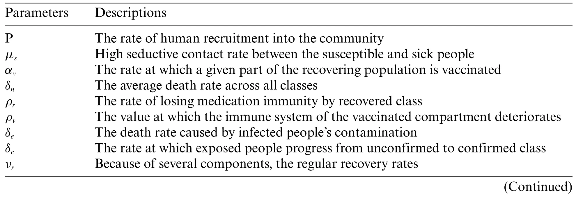
Table 2:Parameters and their descriptions

Table 3:Values of the variables(SQIRV)

Table 4:Values of the variables(SEIQIcRVW)

Considering the given aspects,the SEIQIcRVW delay mathematical model is derived as follows:

whereξ1=δn+k+γi+δc,ξ2=δn+δe+νr+ζ+ωc,ξ3=γr+ηv+δn,ξ4=ζq+γc+ζw+δn,ξ5=δn+ρr+αvandξ6=δn+ρv.

Subject to initial conditions:S(0)=S0,E(0)=E0,I(0)=I0,Q(0)=Q0,Ic(0)=,R(0)=,V(0)=V0.

3.1 Steady State Solutions the Delayed SEIQIcRVW Model

The system (15) is found static,i.e.,the solutions of time independent are obtained.The steady state solutions in the infection free state,whenI=0 is given by

The basic reproduction numberR0is

3.2 Stability Analysis of the Delayed SEIQIcRVW Model

The local stability of the SEIQIcRVW system(15)for the infection-free steady state solution(16)is examined in the next theorem applying Rouche’s theorem.The reproduction numberR0determines the result.

Theorem 3.1.The infection free consistent stateE0(16)is locally asymptotically stable if R0<1 and unstable ifR0>1 for the time delayτ≥0.

Proof.The characteristic equation of system 15,for the equilibrium pointE0,is given by

That isR0<1.Clearly infection free steady stateE0is locally asymptotically stable ifR0<1 whenτ=0.

Letτ >0.In this case,we will use Rouche’s theorem to prove that all roots of the characteristic Eq.(19)cannot intersect the imaginary axis,i.e.,the characteristic equation cannot have pure imaginary roots.

Suppose for the opposite,that is,suppose there existsw∈R such thatλ=wiis a solution of(19).

By equating the real and imaginary part,we get

4ξ1ξ2-w2=4μsγiScosτw,w(ξ1+ξ2)=-4μsγiSsinτw

If R0<1,then μsSγi-ξ1ξ2>0.Hencew2<0,which is a contradiction.

Thus the infection free consistent stateE0is locally asymptotically stable if R0<1 forτ≥0.

Now suppose thatR0>1 from the characteristic polynomial (20),it is enough to consider the term(λ+ξ1+ξ2-).It is easy to see thatC1(0) <0.On the other hand,limλ→+∞C1(λ)=+∞.Therefore,by continuity ofC1(λ),there is at least one positive root of the characteristic Eq.(20).Hence,we conclude thatΣ1is unstable,for anyτ≥0.

The local stability of the SEIQIcRVW system(15)for the infection’s persistent steady state solution(17)is determined using Rouche’s theorem and the Routh-Hurwitz technique in the next theorem.The result is governed by the reproduction numberR0.

Theorem 3.2.If R0>1,then the endemic equilibrium pointE∗is locally asymptotically stable forτ≥0.

Proof.The characteristic equation of system 15,for the equilibrium pointE∗17 is given by

Where the Jacobian matrices of the model at infection persistent steady state solution are

The characteristic equation is

(-δn-λ)(ρvμsI∗e-λτ[(ξ2ξ4kξ5ηv+ξ2ζqδcξ5ηv+ξ4ηγiξ5ηv+ξ3ξ4γiνrs+ξ2ξ4kγrαv+ξ2ζqδcγrαv+ξ4ηγiγrαv+ξ3ξ2δcγcαv)+(ξ2ξ4kηv+ξ2ζqδcηv+ξ4ηγiηv+ξ2kξ5ηv+ξ4kξ5ηv+ζqδcξ5ηv+ηγiξ5ηv+ξ3γiνrαv+ξ4γiνrαv+ξ2kγrαv+ξ4kγrαv+ζqδcγrαv+ηγiγrαv+ξ3δcγcαv+ξ2δcγcαv)λ+(ξ2kηv+ξ4kηv+ζqδcηv+ηγiηv+kξ5ηv+γiνrαv+kγrαv+δcγcαv)λ2+kηvλ3]+(-ξ6-λ)(-ρrμsI∗e-λτ[(ξ3ξ4γiνr+ξ2ξ4kγr+ξ2ζqδcγr+ξ4ηγiγr+ξ3ξ2δcγc)+(ξ3γiνr+ξ4γiνr+ξ2kγr+ξ4kγr+ζqδcγr+ηγiγr+ξ3δcγc+ξ2δcγc)λ+(γiνr+kγr+δcγc)λ2]+(-ξ3-λ)(-ξ4-λ)(-ξ5-λ)(-γiμsS∗e-λτ(-δn-λ)+(-ξ2-λ)(δnξ1+ξ1μsI∗e-λτ+(δn+ξ1+μsI∗e-λτ)x+λ2))))=0.

To check about the stability,consider the second term of the above characteristic equation

whereD0=δn+ξ1+ξ2+ξ3+ξ4+ξ5+ξ6,D1=ξ1+ξ2+ξ3+ξ4+ξ5+ξ6,D2=γi,D3=δnξ3+δnξ1+ξ3ξ1+δnξ2+ξ3ξ2+ξ1ξ2+δnξ4+ξ3ξ4+ξ1ξ4+ξ2ξ4+δnξ5+ξ3ξ5+ξ1ξ5+ξ2ξ5+ξ4ξ5+δnξ6+ξ3ξ6+ξ1ξ6+ξ2ξ6+ξ4ξ6+ξ5ξ6,

D4=ξ1ξ2+ξ1ξ3+ξ1ξ4+ξ1ξ5+ξ1ξ6+ξ2ξ3+ξ2ξ4+ξ2ξ5+ξ2ξ6+ξ3ξ4+ξ3ξ5+ξ3ξ6+ξ4ξ5+ξ4ξ6+ξ5ξ6,D5=γi[δn+ξ3+ξ4+ξ5+ξ6],D6=δn[ξ3ξ1+ξ3ξ2+ξ1ξ2+ξ3ξ4+ξ1ξ4+ξ2ξ4+ξ3ξ5+ξ1ξ5+ξ2ξ5+ξ4ξ5+ξ2ξ6+ξ3ξ6+ξ1ξ6+ξ4ξ6+ξ5ξ6]+ξ3ξ4ξ5+ξ1ξ4ξ5+ξ2ξ4ξ5+ξ3ξ1ξ2+ξ3ξ1ξ6+ξ3ξ2ξ6+ξ3ξ2ξ4+ξ3ξ2ξ5+ξ1ξ2ξ5+ξ1ξ2ξ4+ξ3ξ1ξ4+ξ1ξ2ξ6+ξ3ξ1ξ5+ξ3ξ4ξ6+ξ1ξ4ξ6+ξ2ξ4ξ6+ξ3ξ5ξ6+ξ1ξ5ξ6+ξ2ξ5ξ6+ξ4ξ5ξ6,

D7=ξ3ξ1ξ2+ξ3ξ1ξ2+ξ3ξ2ξ4+ξ1ξ2ξ4+ξ3ξ1ξ5+ξ3ξ2ξ5+ξ1ξ2ξ5+ξ3ξ4ξ5+ξ1ξ4ξ5+ξ2ξ4ξ5+ξ3ξ1ξ6+ξ3ξ2ξ6+ξ1ξ2ξ6+ξ3ξ4ξ6+ξ1ξ4ξ6+ξ2ξ4ξ6+ξ3ξ5ξ6+ξ1ξ5ξ6+ξ2ξ5ξ6+ξ4ξ5ξ6-ρrγiνr-ρrkγr-ρrδcγc-ρvkηv,D8=γi[ξ3ξ4+δnξ5+ξ3ξ5+δnξ6+ξ3ξ6+ξ4ξ6+ξ5ξ6+δnξ3+ξ4ξ5+δnξ4],D9=ξ3ξ1ξ2ξ4+δnξ3ξ1ξ2+δnξ3ξ1ξ4+δnξ3ξ2ξ4+δnξ1ξ2ξ4+δnξ3ξ1ξ5+δnξ3ξ2ξ5+δnξ1ξ2ξ5+ξ3ξ1ξ2ξ5+δnξ3ξ4ξ5+δnξ1ξ4ξ5+ξ3ξ1ξ4ξ5+δnξ2ξ4ξ5+ξ3ξ2ξ4ξ5+ξ1ξ2ξ4ξ5+δnξ3ξ1ξ6+δnξ3ξ2ξ6+δnξ1ξ2ξ6+ξ3ξ1ξ2ξ6+δnξ3ξ4ξ6+δnξ1ξ4ξ6+ξ3ξ1ξ4ξ6+δnξ2ξ4ξ6+ξ3ξ2ξ4ξ6+ξ1ξ2ξ4ξ6+δnξ3ξ5ξ6+δnξ1ξ5ξ6+ξ3ξ1ξ5ξ6+δnξ2ξ5ξ6+ξ3ξ2ξ5ξ6+ξ1ξ2ξ5ξ6+δnξ4ξ5ξ6+ξ3ξ4ξ5ξ6+ξ1ξ4ξ5ξ6+ξ2ξ4ξ5ξ6,

D10=ξ3ξ1ξ2ξ4+ξ3ξ1ξ2ξ5+ξ3ξ1ξ4ξ5+ξ3ξ2ξ4ξ5+ξ1ξ2ξ4ξ5+ξ3ξ1ξ2ξ6+ξ3ξ1ξ4ξ6+ξ3ξ2ξ4ξ6+ξ1ξ2ξ4ξ6+ξ3ξ1ξ5ξ6+ξ3ξ2ξ5ξ6+ξ1ξ2ξ5ξ6+ξ3ξ4ξ5ξ6+ξ1ξ4ξ5ξ6+ξ2ξ4ξ5ξ6-ξ3ρrγiνr-ρrξ4γiνr-ρrξ2kγr-ρrξ2kγr-ρrζqδcγr-ρrηγiγrξ3ρrδcγc-ρrξ2δcγc-ρvξ2kηv-ρvξ4kηv-ρvζqδcηv-ρvηγcηv-ρvkξ5ηv-ρvγiνrαv-ρvkγrαv-ρvδcγcαv-ρrγiνrξ6-ρrkγrξ6-ρrδcγcξ6,D11=γi[δnξ3ξ4+δnξ3ξ5+δnξ4ξ5+ξ3ξ4ξ5+δnξ3ξ6+δnξ4ξ6+ξ3ξ4ξ6+δnξ5ξ6+ξ3ξ5ξ6+ξ4ξ5ξ6],D12=δnξ3ξ1ξ2ξ4+δnξ3ξ1ξ2ξ5+δnξ3ξ1ξ4ξ5+δnξ3ξ2ξ4ξ5+δnξ1ξ2ξ4ξ5+ξ3ξ1ξ2ξ4ξ5+δnξ3ξ1ξ2ξ6+δnξ3ξ1ξ4ξ6+δnξ3ξ2ξ4ξ6+δnξ1ξ2ξ4ξ6+ξ3ξ1ξ2ξ4ξ6+δnξ3ξ1ξ5ξ6+δnξ3ξ2ξ5ξ6+δnξ1ξ2ξ5ξ6+ξ3ξ1ξ2ξ5ξ6+δnξ3ξ4ξ5ξ6+δnξ1ξ4ξ5ξ6+ξ3ξ1ξ4ξ5ξ6+δnξ2ξ4ξ5ξ6+ξ3ξ2ξ4ξ5ξ6+ξ1ξ2ξ4ξ5ξ6,

D13=ξ3ξ1ξ2ξ4ξ5+ξ3ξ1ξ2ξ4ξ6+ξ3ξ1ξ2ξ5ξ6+ξ3ξ1ξ4ξ5ξ6+ξ3ξ2ξ4ξ5ξ6+ξ1ξ2ξ4ξ5ξ6-ξ3ρrξ4γiνr-ρrξ2ξ4kγrρrξ2ζqδcγr-ρrξ4ηγiγr-ξ3ρrξ2δcγc-ρvξ2ξ4kηv-ρvξ2ζqδcηv-ρvξ4hγiηv-ρvξ2kξ5ηv-ρvξ4kξ5ηv-ρvζqδcξ5ηvρvηγiξ5ηv-ξ3ρvγiνrαv-ρvξ4γiνrαv-ρvξ2kγrαv-ρvξ4kγrαv-ρvζqδcγrαv-ρvηγiγrαv-ξ3ρvδcγcαv-ρvξ2δcγcαvξ3ρrγiνrξ6-ρrξ4γiνrξ6-ρrξ2kγrξ6-ρrξ4kγrξ6-ρrζqδcγrξ6-ρrηγiγrξ6-ξ3ρrδcγcξ6-ρrξ2δcγcξ6,

D14=γi[δnξ3ξ4ξ5+δnξ3ξ4ξ6+δnξ3ξ5ξ6+δnξ4ξ5ξ6+ξ3ξ4ξ5ξ6],D15=δnξ3ξ1ξ2ξ4ξ5+δnξ3ξ1ξ2ξ4ξ6+δnξ3ξ1ξ2ξ5ξ6+δnξ3ξ1ξ4ξ5ξ6+δnξ3ξ2ξ4ξ5ξ6+δnξ1ξ2ξ4ξ5ξ6+ξ3ξ1ξ2ξ4ξ5ξ6,

D16=ρvξ2ξ4kξ5ηv+ξ3ξ1ξ2ξ4ξ5ξ6-ρvξ2ζqδcξ5ηv-ρvξ4ηγiξ5ηv-ξ3ρvξ4γiνrαv-ρvξ2ξ4kγrαv-ρvξ2ζqδcγrαvρvξ4ηγiγrαv-ξ3ρvξ2δcγcαv-ξ3ρrξ4γiνrξ6-ρrξ2ξ4kγrξ6-ρrξ2ζqδcγrξ6-ρrξ4ηγiγrξ6-ξ3ρrξ2δcγcξ6,D17=γiδnξ3ξ4ξ5ξ6,D18=δnξ1ξ2ξ2ξ4ξ5ξ6.

Ifτ=0,then by using the rule of Descartes of sign,we can get there are no positive real roots.

Also by Routh-Hurwitz stability criterion,the real parts of the complex roots are also negative ifμsI∗(ξ1+ξ2+ξ3+ξ4+ξ5+ξ6)-μsS∗γi+D3>0,(1-R0)<0,R0>1.Then the infection persistent steady state(S∗,E∗,I∗,Q∗,I∗c,R∗,V∗,W∗)is locally stable when R0<1.

Ifτ >0,then by using Rouche’s theorem,we have to prove that all roots of the characteristic Eq.(22) cannot have pure imaginary roots.Suppose that there existsw∈R such thatλ=wiis a solution of(22).Now Eq.(22)becomes

Squaring both Eqs.(26),(27)and adding,we get

Letz=w2in(27)

If R0>1,then from Eq.(28),we can see that()is strictly positive which impliesF(0)<0.Thus,we can get atleast one positive real root.Hence,if R0>1 all the real parts of the roots of(22)are negative.Thus,the equilibrium positionE∗is stable when R0>1 forτ≥0.

4 Numerical Analysis

During the second wave of the Corona virus,India experienced a high infection rate.We obtained data for this article from Tamilnadu,India.This current Omicron variant pandemic data of Tamilnadu,India is validated with our theoretical findings.The source of the data is specified by[28] and [23].Tamil Nadu encountered its most memorable instance of the Omicron type of SARSCoV-2 on December 15,2021,as indicated by a traveller from another country.Three weeks after the first confirmed Omicron case was reported,Tamil Nadu was infected with the highly transmissible and rapidly spreading form of SARS-Cov-2.The data for this study is gathered from the state of Tamil Nadu (Chennai).As of March 11,2022,there were 750606 positive cases,750520 discharged cases,48 deaths,499 active cases,42 positive cases on March 11,2022,86 recovered cases,and 3373 vaccinated cases.The state of Tamilnadu achieves a zero-death rate and a safe position against the spread of Omicron on March 11,2022.We used Mathematica for plotting the solution.The values of the variables and parameters are listed in the Tables 3 and 4 below.

The susceptible individual curves for the systems SEIQIcRVW and SQIRV are depicted in Figs.1–3,respectively.For the system SEIQIcRVW,we used the delay values(τ)0.11,0.14,and 0.16,and for the system SQIRV,we used the delay values(τ)0.002,0.003,and 0.004.

Figure 1:Susceptible people S(t)against time t with various τ for SEIQIcRVW

Figure 2:Susceptible people S(t)against time t with various τ for SQIRV

Fig.4 demonstrates that when the exposed population decreases,the population of other compartments also decreases,while when the exposed population rises,the population of all related compartments rises.

Figs.5–7 illustrate the possible reduction in the Omicron infection rate.Fig.5 demonstrates that when the Omicron variant was first discovered,its spread was rapid,and that the variant’s spread was reduced to a safe level when the government implemented quarantine and vaccination at a high rate.By adding more compartments from the models that came before it,the SEIQIcRVW model is able to keep the increase in infected individuals under control at a moderate rate.The state of Tamilnadu discovered on March 11,2022,that Omicron’s death had not been caused by anyone.People were able to avoid contracting the SARS Cov-2 Omicron variant through vaccination against COVID-19.

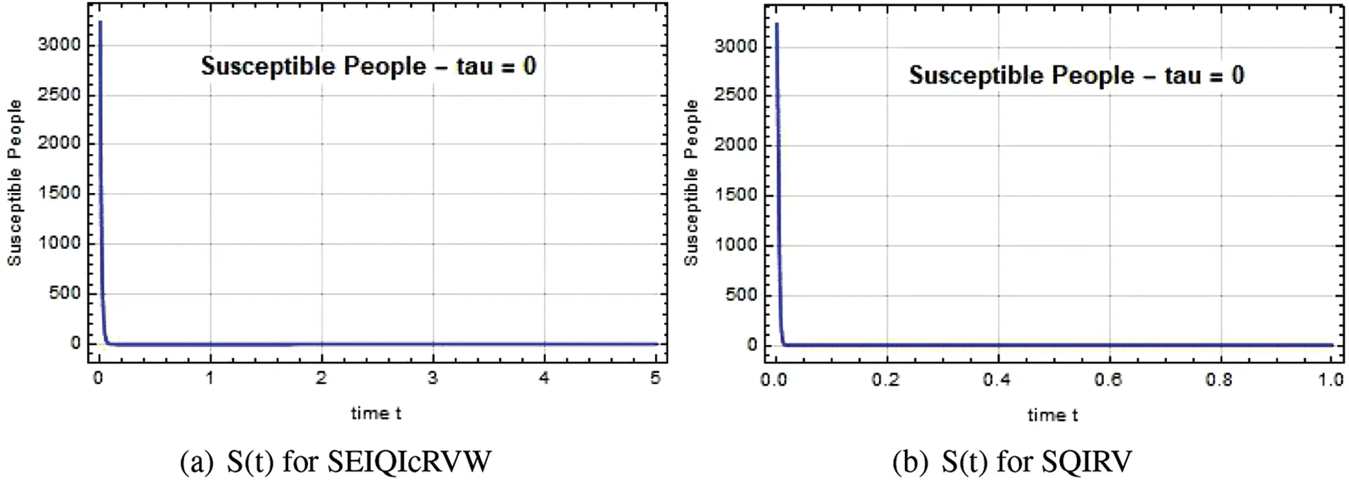
Figure 3:Susceptible people S(t)against time t with τ=0 for SEIQIcRVW and SQIRV

Figure 4:Exposed people E(t)against time t with various τ for SEIQIcRVW

Figure 5:Infected people I(t)against time t with various τ for SEIQIcRVW

Figure 6:Infected people I(t)against time t with various τ for SQIRV

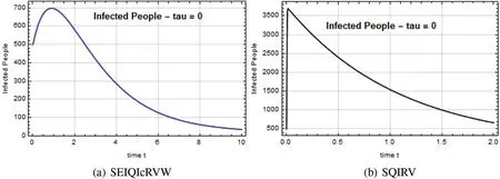
Figure 7:Infected people I(t)against time t with τ=0 for SEIQIcRVW and SQIRV

The Quarantined individual level at time t is depicted in Figs.8–10.When the government implemented the quarantine in Chennai at a high range,the spread of the disease was contained,and the situation in Chennai returned to normal.

Figure 8:Quarantined people Q(t)against time t with various τ for SEIQIcRVW

Figure 9:Quarantined people Q(t)against time t with various τ for SQIRV

According to Fig.11,the population of these four districts experiences a high rate of illness during the Omicron period,which begins on December 25 and ends on March 11,2022.The infection rate gradually decreased to a low level and there were no deaths when people were vaccinated in accordance with government instructions.

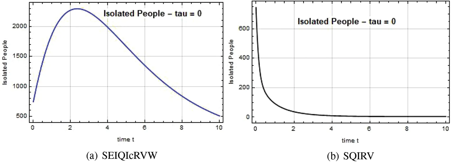
Figure 10:Quarantined people Q(t)against time t with τ=0 for SEIQIcRVW and SQIRV

Figure 11:Confirmed people S(t)against time t with various τ for SEIQIcRVW

Reproduction numbers of 0.66,0.92,0.63,and 0.06 for SEIQIcRVW and 0.02,0.05,0.073,and 0.074 for SQIRV are shown in Fig.12.Contaminations are being eliminated from the host population when R0<1.However,ifR0>1,the contaminations cause harm and become endemic,necessitating appropriate clinical treatments to stop the spread of the disease.If the delay valueτ=0.014 for the system SEIQIcRVW andτ=0.003 for the system SQIRV,prominent oscillation is observed in the infected population.This could be interpreted as indicating that even though people recover over time,oscillations indicate that the exposed or asymptomatic population has a higher number of active cases than the infected population.

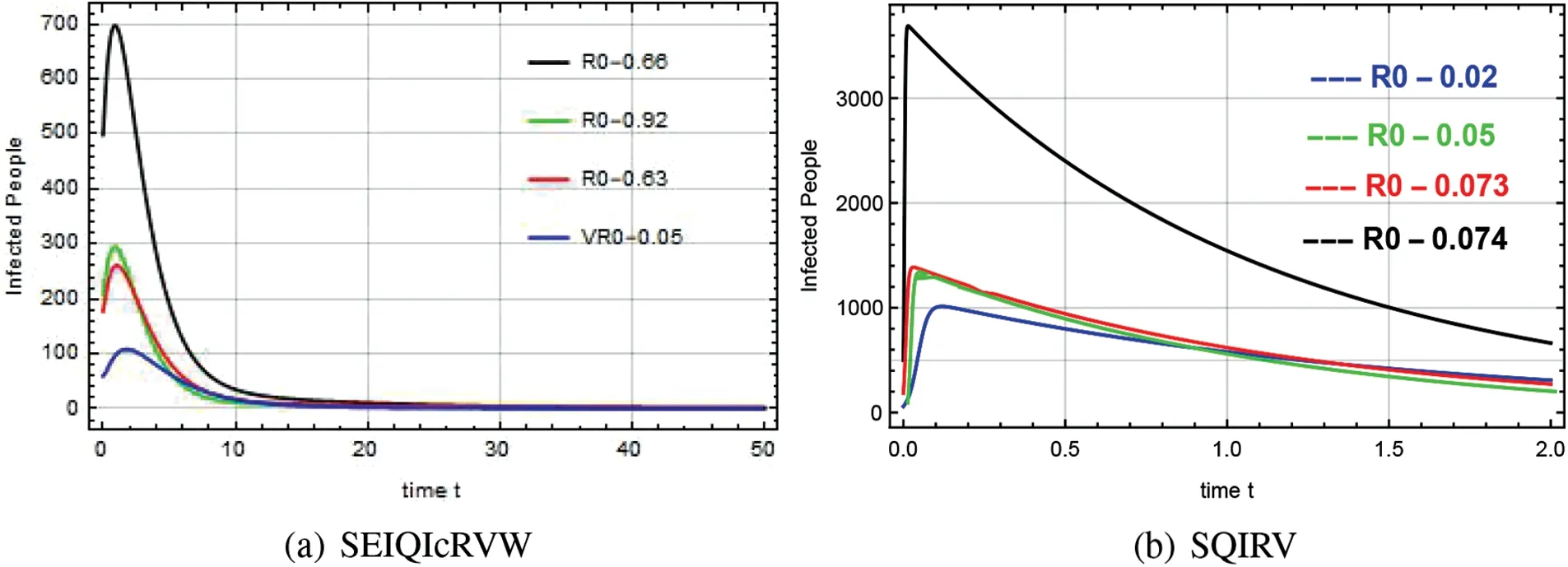
Figure 12:Infected range about various reproduction numbers for the system SEIQIcRVW and SQIRV

The rise in recovered rates for both systems in Chennai is depicted in Figs.13–15.By balancing the recovered and infected rates with standard rates,the system SEIQIcRVW achieves stability.

Figure 13:Recovered people R(t)against time t with various τ for SEIQIcRVW

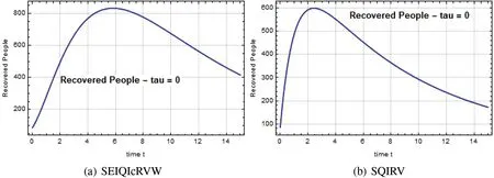
Figure 15:Recovered people R(t)against time t with τ=0 for SEIQIcRVW and SQIRV

The rapid rise in the number of people being vaccinated is depicted in Figs.16–18.As a result,the system’s infection rate significantly decreased,and the system became stable.The significance of vaccination to the Omicron virus control strategy is demonstrated by these figures.

The effect of delayed SEIQIcRVW model construction is depicted in Fig.19 as a decrease in reservoir individuals over time t.Figs.20 and 21 show the stability of the Omicron mathematical model for the Chennai district at various delay values.The infection rate decreases for both the SEIQIcRVW and SQIRV systems following a rapid spread over a considerable period,as shown in Fig.22.These systems control the infection and stop its spread within a few days.

Figure 16:Vaccinated people V(t)against time t with various τ for SEIQIcRVW

Figure 17:Vaccinated people V(t)against time t with various τ for SQIRV

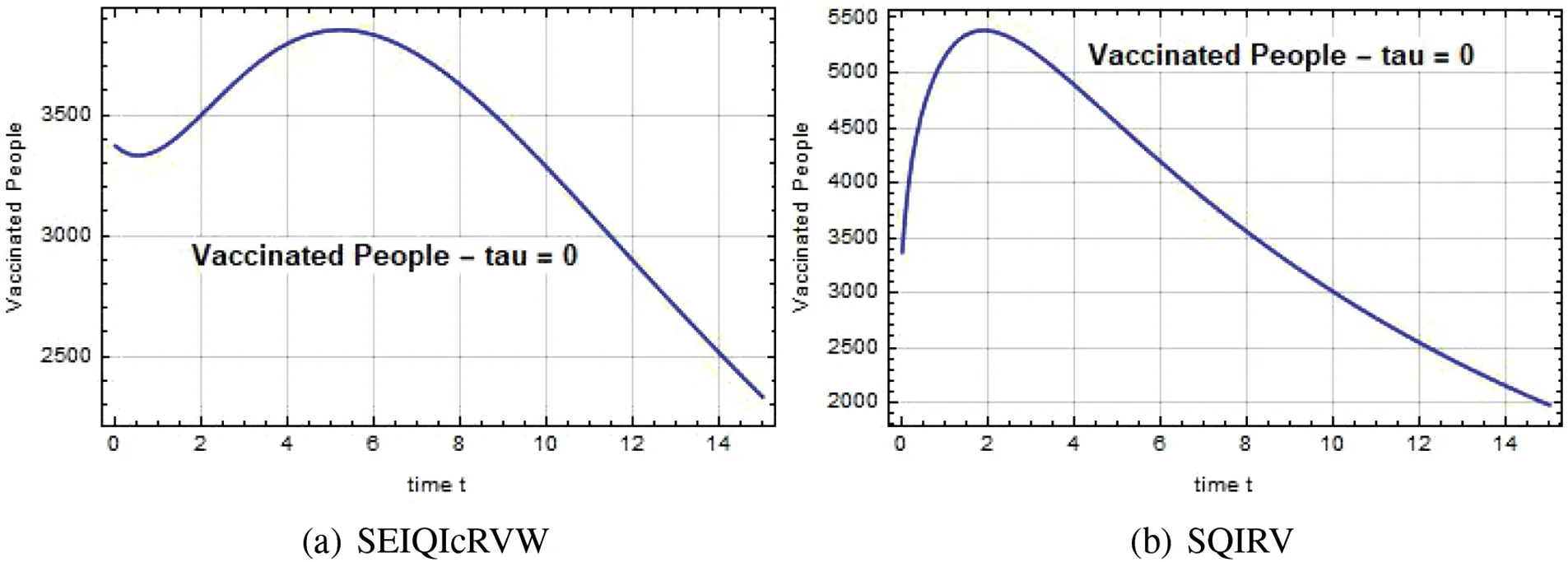
Figure 18:Vaccinated people V(t)against time t with τ=0 for SEIQIcRVW and SQIRV

Figure 19:Reservoir people W(t)against time t with various τ for SEIQIcRVW

Figure 20:Stability of the system SEIQIcRVW against time t with various τ

Figure 21:Stability of the system SQIRV against time t with various τ

Figure 22:Stability of the systems with τ=0

5 Conclusions

Novel delayed mathematical models for the Omicron B.1.1.529 SARS-Cov-2 Variant were developed in this paper.The stability of the two models has been examined and validated,and the principles of reproduction number calculated with this model are an outbreak threshold that determined whether or not the disease would spread further in the district Chennai of Tamilnadu.As the figures show,infection-free steady-state solutions are locally asymptotically stable when R0<1.The derived solutions show that the systems are locally unstable and will never become stable whenR0>1 for an infection-free steady state.From all the data,we can say that the host community will be safe from the Omicron variant if more people are isolated,recovered,and vaccinated.We also found that the second wave of SARS Cov-2 Omicron variant spreads less if the intercessions are strictly followed.Based on our mathematical models and the Chennai data,the Omicron variant infection appears to have stabilized after approximately 25 days.This study will be beneficial for scientists who are working in the medical field.This work can be further extended to generalize with different fractional derivative models.

Acknowledgement:This study is supported via funding from Prince Sattam bin Abdulaziz University Project Number (PSAU/2023/R/1444).The first author is partially supported by the University Research Fellowship(PU/AD-3/URF/21F37237/2021 dated 09.11.2021)of Periyar University,Salem.The second author is supported by the fund for improvement of Science and Technology Infrastructure(FIST)of DST(SR/FST/MSI-115/2016).

Funding Statement:This study is supported via funding from Prince Sattam bin Abdulaziz University Project Number (PSAU/2023/R/1444).The first author is partially supported by the University Research Fellowship(PU/AD-3/URF/21F37237/2021 dated 09.11.2021)of PeriyarUniversity,Salem.The second author is supported by the fund for improvement of Science and Technology Infrastructure(FIST)of DST(SR/FST/MSI-115/2016).

Author Contributions:S.Dickson: Conceptualization,Visualization,Software,Resources,Formal analysis,Investigation,Writing-original draft.S.Padmasekaran: Investigation,Supervision,Formal analysis,Writing-review &editing.P.Kumar: Investigation,Supervision,Formal analysis,Writingreview &editing.Kottakkaran Sooppy Nisar: Investigation,Supervision,Formal analysis,Writingreview &editing.Hamidreza Marasi: Investigation,Supervision,Formal analysis,Writing-review &editing.

Availability of Data and Materials:Data sharing not applicable to this article as no datasets were generated or analyzed during the current study.

Conflicts of Interest:The authors declare that they have no conflicts of interest to report regarding the present study.