Detecting the presence of natural forests using airborne laser scanning data

Marie-Claude Jutras-Perreault, Terje Gobakken, Erik Næsset, Hans Ole Ørka

Faculty of Environmental Sciences and Natural Resource Management, Norwegian University of Life Sciences, NMBU, P.O.Box, NO-1432 Ås, Norway

Keywords:Natural forest ALS Naturalness Vertical variables Horizontal variables Biodiversity Forest condition Ecosystem services

ABSTRACT Centuries of forest exploitation have caused significant loss of natural forests in Europe, leading to a decline in populations for many species.To prevent further loss in biodiversity,the Norwegian government has set a target of protecting 10%of the forested area.However,recent data from the National Forest Inventory(NFI)reveals that less than 2%of Norway's forested area consists of natural forests.To identify forests with high conservation value,we used vertical and horizontal variables derived from airborne laser scanning (ALS) data, along with NFI plot measurements.Our study aimed to predict the presence of natural forests across three counties in southeastern Norway, using three different definitions: pristine, near-natural, and semi-natural forests.Natural forests are scarce, and their underrepresentation in field reference data can compromise the accuracy of the predictions.To address this,we assessed the potential gain of including additional field data specifically targeting natural forests to achieve a better balance in the dataset.Additionally, we examined the impact of stratifying the data by dominant tree species on the performance of the models.Our results revealed that semi-natural forests were the most accurately predicted, followed by near-natural and pristine forests, with Matthews correlation coefficient values of 0.32, 0.24, and 0.17, respectively.Including additional field data did not improve the predictions.However,stratification by species improved the accuracy of predictions for near-natural and semi-natural forests,while reducing accuracy for pristine forests.The use of horizontal variables did not improve the predictions.Our study demonstrates the potential of ALS data in identifying forests with high conservation value.It provides a basis for further research on the use of ALS data for the detection and conservation of natural forests, offering valuable insights to guide future forest preservation efforts.

1.Introduction

After centuries of forest exploitation, very few forests unaffected by human activity remain in Scandinavia (Gjerde et al., 2007; Tomter and Dalen,2014).Initially,logging intensity varied based on the proximity to rivers suitable for timber floating.However, with the expansion of the forest road network, remote forest areas became more accessible.The reduction of natural forests and deadwood abundance has led to significant population declines for numerous species in Fennoscandia(Edman et al.,2004; Penttil¨a et al.,2006;Stokland and Kauserud,2004).

To limit further loss in biodiversity, the Norwegian government has set a target for protecting 10% of the forested area (Stortinget, 2016).Similarly, new standards for forest certification from the Program for Endorsement of Forest Certification(PEFC)require that 5%of productive forests larger than 1,000 ha be set aside as biologically important areas for conservation value(PEFC Norway,2022).However,according to the latest National Forest Inventory (NFI) campaign, natural forests only cover 1.7%of the forested area in Norway(Framstad et al.,2016).

The Norwegian NFI's definition of natural forest,hereafter referred to as “pristine forests”, includes forests that have maintained their ecological integrity, vegetation diversity and structure, and ecological processes, without significant disturbance from human activity (Rolstad et al.,2002;Viken,2018;Storaunet and Rolstad,2020).However,due to the limited availability of pristine forests,other forests with high levels of naturalness need to be considered as a viable alternative for conservation purposes (Søgaard et al., 2012).Selective felling of valuable species of large diameter followed by natural regeneration was a common practice in Norway until the mid-twentieth century when it was gradually replaced by clear-cutting and planting (Storaunet et al., 2005).Old forests having evolved from abandoned selectively logged areas, hereafter referred to as“near-natural”and“semi-natural”forests,exhibit a higher degree of naturalness, with more complex within-stand vertical and horizontal structures than old forests resulting from clear-cutting, hereafter referred to as “managed forests”.Near-natural and semi-natural forests present a larger variation in tree size and age structure than managed forests (Siitonen, 2001).They often follow a reversed J-shape diameter distribution(Linder et al.,1997)and contain a greater amount of deadwood (Siitonen, 2001; Stokland et al., 2004).Additionally, they present more gaps caused by natural disturbances such as fire, windstorms, or damage from snow or ice than managed forests and a higher number of deciduous trees (Esseen et al., 1997).These forests are associated with higher biodiversity(Paillet et al.,2010)and are highly valued habitats for many red-listed and endangered species (Tikkanen et al.,2006;Stokland and Larsson,2011; Magnusson et al., 2014).

Combining remotely sensed data with field reference data can be an effective and systematic approach to identify and delineate forests with high conservation value.Airborne laser scanning(ALS)data can provide information on the horizontal and vertical distribution of biological material, enabling a comprehensive characterization of the threedimensional structure of the forest canopy.The use of ALS data as a tool for assessing various forest attributes has gained popularity worldwide,and full coverage of ALS data for forests is now available in many countries.

Although only a few studies have focused on the detection of natural forests using remotely sensed data, many have explored elements associated with natural forests, such as vertical and horizontal complexity and the presence of gaps and dead trees.Various methods have been used to characterize the vertical canopy structure,including quantiles of ALS height distribution (Maltamo et al., 2005), ALS-derived tree height variance(Zimble et al.,2003),and standard deviation and coefficient of variation of ALS point heights (Blaschke et al., 2004).Horizontal complexity has been mainly assessed through gap patterns.While some studies have delineated gaps directly on the ALS point clouds (Gaulton and Malthus,2010),most have used a fixed height threshold on canopy height models(CHM)derived from ALS data to identify openings in the forest canopy (Bonnet et al., 2015).However, variations were observed among studies in the CHM spatial resolution,the specific threshold value used,and the requirement for a minimum area constraint(Koukoulas and Blackburn, 2004; Vepakomma et al., 2008; Kane et al., 2011; Vehmas et al., 2011).Concerning deadwood, ALS-derived metrics of height and density have been used to estimate the distribution of standing dead trees in different stages of decay(Bater et al.,2009)and to assess the presence of snags (Martinuzzi et al., 2009), while ALS-derived metrics of height and intensity of the signal have been used to predict the volume of standing and downed dead trees(Pesonen et al.,2008).

ALS data have proven to be an effective tool for predicting forest stand age, maturity, and naturalness.For instance, Schumacher et al.(2020) used NFI data, upper percentiles of ALS heights, and Sentinel-2 data to predict forest stand age, achieving a RMSE of 3-31 years depending on the site index value.Martin and Valeria(2022)successfully distinguished old-growth forests in early and late succession stages using ALS structural indices such as height percentiles,coefficient of variation,and gap fraction derived from CHM at 1 m spatial resolution, with an error rate of 4.9%.Sverdrup-Thygeson et al.(2016) used ALS data to distinguish between old natural and old managed forests.While this study found that the most important metrics were related to canopy height and density,variation in the canopy height,tree density,and gap patterns, they concluded that the horizontal metrics outperformed the vertical metrics in terms of accuracy.Fuhr et al.(2022) developed a maturity index based on the basal area and volume of large trees and deadwood, decay stage, and species diversity.To predict the level of maturity, they employed vertical, horizontal, and intensity metrics derived from ALS data, along with topographic metrics.The resulting maturity index values ranged from 0 to 1.Despite obtaining high RMSE values of 1.26 for validation data,the study revealed a strong correlation(0.89) between the observed and predicted maturity index value.The value of old forests was predicted using an index developed from field-measured forest structural attributes and ALS-derived metrics (de Assis Barros and Elkin, 2021).Similarly, Huo et al.(2023) defined the conservation value of forests based on the number of standing dead trees,downed dead trees, and important trees for biodiversity conservation.They achieved a R2value of 0.60 for the predicted conservation values at the plot level, with detection error rates of 52%, 71%, and 83% for the respective tree categories.

As natural forests are rare, they are often underrepresented in field reference data, including NFI data.This can lead to underestimation of probabilities when performing logistic regression using an unbalanced dataset, which can compromise the accuracy of the results (King and Zeng, 2001).We hypothesize that increasing the amount of field data containing information about natural forests could improve the accuracy of our results.Furthermore,given that the vertical forest structure varies depending on species composition, we also propose that stratifying the data by dominant tree species could further refine the accuracy of our models.To the authors’ knowledge, no previous studies have explored the potential gains of incorporating additional field reference data into NFI data for the detection of natural forests, nor have they investigated the stratification of data by dominant tree species for a large area.

In this study, we assessed the potential of ALS data in conjunction with plot measurements from standard sampling inventory procedures to detect the presence of natural forests in southeastern Norway.More specifically,the objectives were to:

1) Assess the accuracy of ALS data in combination with NFI data to predict the presence of natural forests;

2) Evaluate the potential gain in model prediction performance achieved by incorporating additional data containing information about natural forests alongside NFI data;

3) Evaluate the potential gain in model prediction performance achieved through stratification based on dominant tree species.

2.Material and methods

2.1.Study area

The study was conducted in southeastern Norway,in the counties of Oslo,Vestfold and Telemark,and Viken(Fig.1).Together,these counties cover approximately 40,000 km2,of which around 32%is forested.Most of the forested areas are found in valleys and are composed of Norway spruce (Picea abies (L.) Karst.), Scots pine (Pinus sylvestries L.), birch species(Betula pendula Roth and B.pubescens Ehrh),and other deciduous trees.Forests can be found at elevations ranging from sea level up to approximately 1,200 m at the alpine treeline.Fig.1 also depicts the locations of plots sampled in old forests (cf.section 2.2 for a full description),along with the vertical profiles of ALS point clouds in managed and natural forest stands.

2.2.Ground reference data

Field data from three datasets were used in this study: 2,098 permanent NFI plots,113 permanent NFI plots in protected areas,and 237 additional plots located in old forests.For certain plots,it was not feasible to calculate some of the variables derived from remotely sensed data.For this reason, the final number of plots employed in the study comprised 2,043 permanent plots,112 permanent plots in protected areas,and 236additional plots located in old forests (cf.sections 2.4.1 and 2.4.3 for a full description).The permanent plots were established between 1986 and 1993 and were resampled during five subsequent inventory cycles.The measurements from the most recent inventory cycle, from 2015 to 2019,were retained,except for plots that were harvested.In the event of harvest, the measurements from the most recent inventory conducted prior to harvest were retained.In natural reserves with forest as a conservation theme,the network of sample plots was densified as part of the NFI from 2012 to 2016, resulting in additional plots sampled 1.5 km north and 1.5 km east of a permanent plot located in a protected area(Viken,2018).The third dataset, collected in 2020,included additional plots that were spread across old forests in the counties.The selection of these plots was based on existing mapping of old high conservation value forests(Direktoratet for naturforvaltning engl.:Norwegian Directorat for Nature Management, 2007).

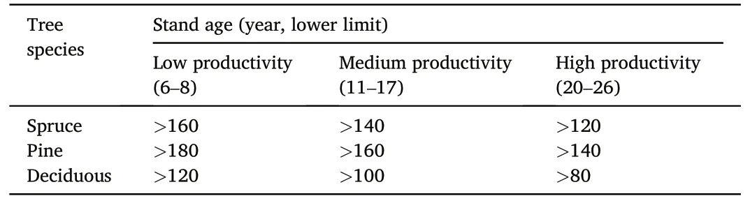
Table 1Minimum age threshold requirement for near-natural forests for different tree species and productivity classes based on the H40 site index system (Søgaard et al.,2012).

For the three field datasets, circular plots of size 250 m2were measured following standard field procedures of the Norwegian NFI(Viken,2018).All living and standing dead trees with diameter at breast height(DBH)of ≥5 cm were measured,and their species and status,i.e.,living or dead,were recorded.The height of approximately 10 trees per plot selected with probability proportional to stem basal area was measured.The height of the two largest trees in terms of DBH was measured and their age was determined using core sampling.For the permanent plots and the permanent plots in protected areas, the two trees were selected outside the 250 m2plot boundary but within a 1,000 m2range.The tree selection for the additional plots in old forests was confined within the boundaries of the 250 m2plots.The chosen trees were spruce, pine, or birch belonging to the dominant tree species and not substantially older than the rest of the trees in the stand.The type of forest, whether pristine or managed, was recorded (cf.section 2.4 for a full description).

For each plot,the total basal area of all living trees and the total basal area of living spruce,pine,and other deciduous trees,respectively,were calculated.Plots with 70% or more of basal area composed of spruce were classified as spruce-dominated, while those with 70% or more of basal area composed of pine were classified as pine-dominated.If neither of these criteria were met, the plots were classified as mixed.For the additional plots in old forests,site index was predicted using the age and height of the two largest dominant trees in the plot by adopting the H40 site index system based on age-height curves of the expected height of the dominant tree species at stand level at the index age of 40 years(Tveite,1977).If other deciduous trees besides birch were selected,birch curves were used(Braastad,1966).For plots with more than one tree sampled,the age and the site index were averaged for trees of the same species.When a spruce or a pine was sampled together with a birch,only the age and the site index of the spruce or the pine were considered.Development class was determined based on age, species, and site index, with younger production forests classified as class III,older production forests as class IV,and old forests as class V(Steinset,1999).For the permanent plots and the permanent plots in protected areas, the site index and development class were registered on-site during the NFI inventory.The site index was predicted using the age and height of the two largest dominant trees located outside the plot but within a 1,000 m2range,using the H40 site index system.

2.3.Natural forest definitions

In this study, pristine forests are defined in accordance with the Norwegian NFI criteria for natural forests.These forests exhibit no visible signs of encroachment and cover an area greater than 0.5 ha, thereby preserving the natural character of the forest(Viken,2018).They contain native tree species,including old trees,and have a multi-layered vertical structure,with deadwood at various stages of decay,including large dimensions.Plantation forests, in contrast, have over 90% of trees belonging to a single species and age class,while managed forests do not meet the criteria of natural or plantation forests.None of the datasets used in this study contained any plantations.The forest type is recorded on-site.

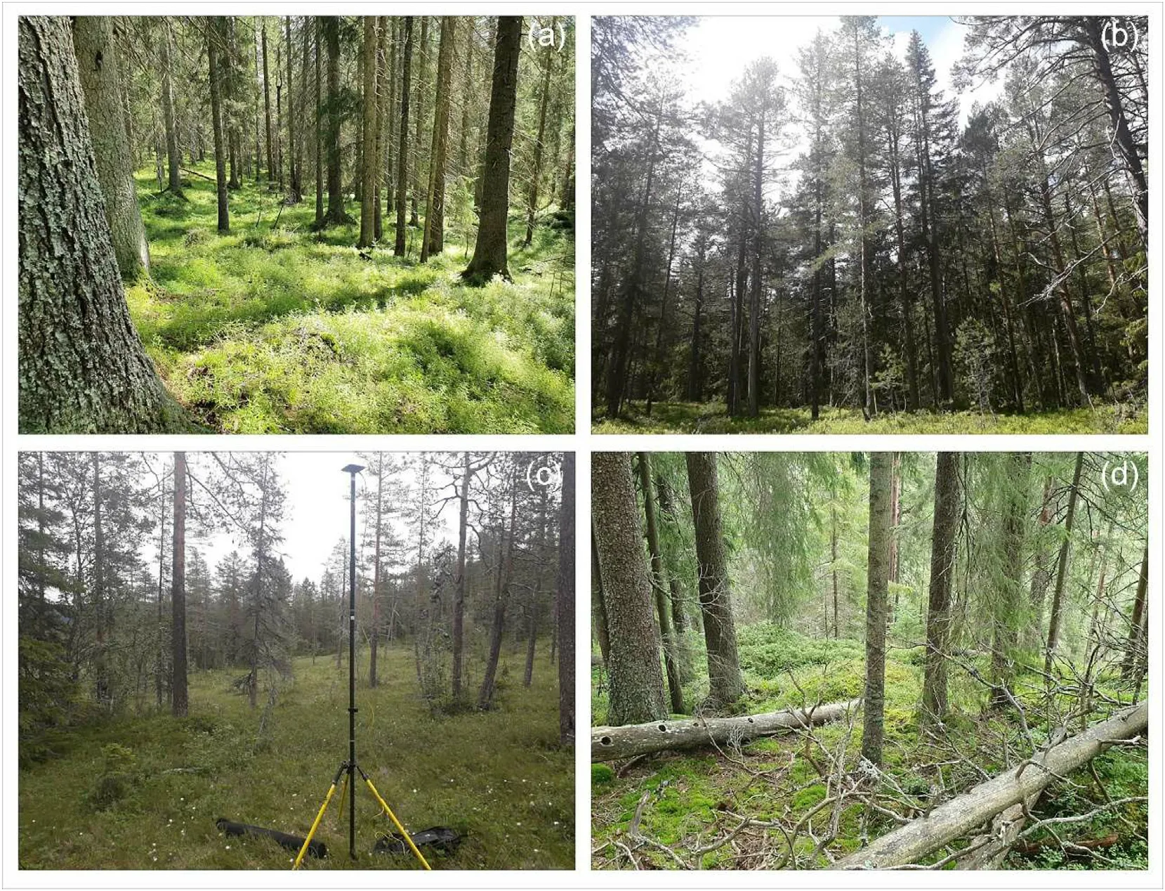
Fig.2.Photos of managed (a), semi-natural (b), near-natural (c), and pristine (d) forest stands located in southeastern Norway.

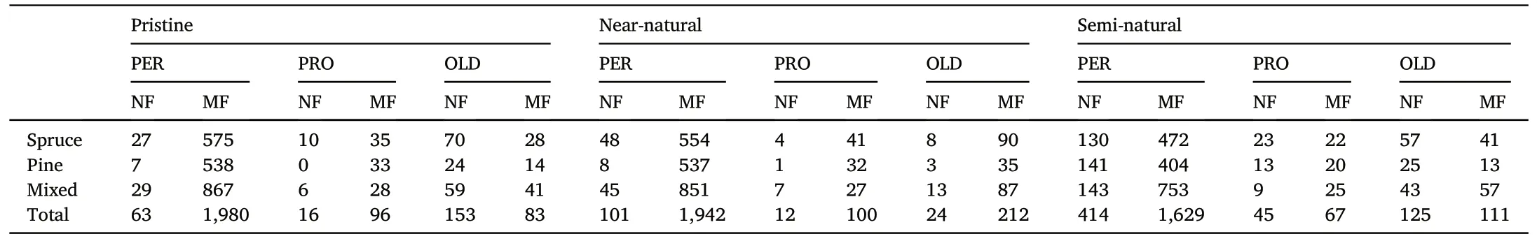
Table 2Number of plots stratified by dominant tree species classified as natural forests(NF)and managed forests(MF)according to three different definitions of natural forests(pristine, near-natural, and semi-natural) for each dataset (PER: permanent plots, PRO:permanent plots in protected areas,OLD: additional plots in old forests).

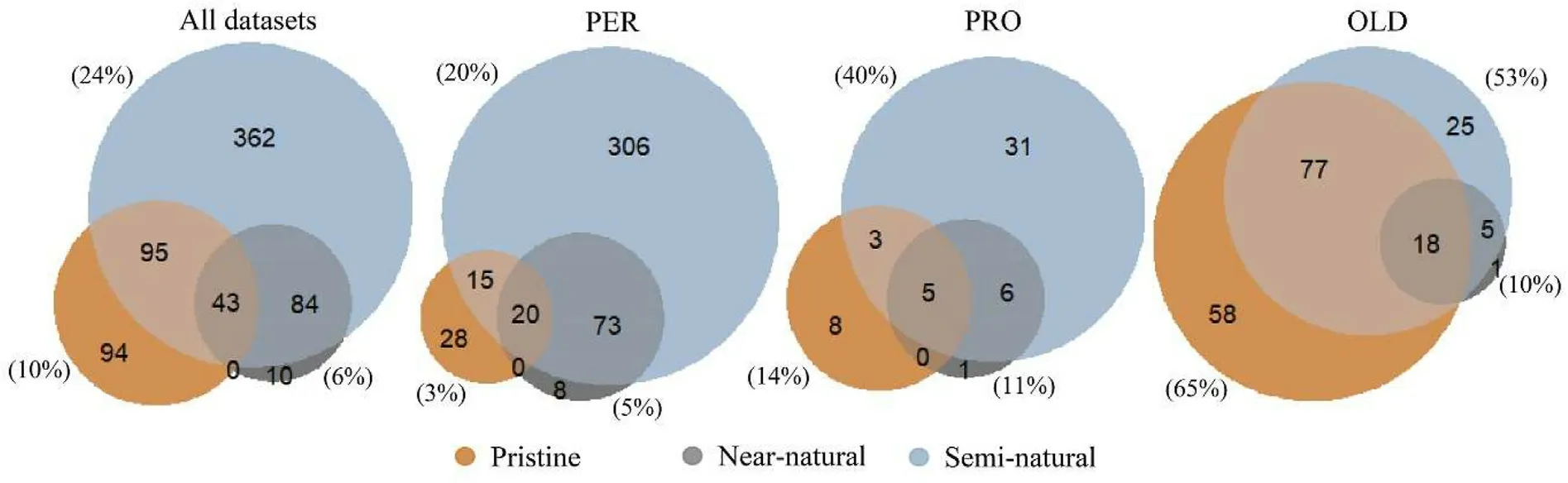
Fig.3.Number of plots defined as pristine, near-natural, and semi-natural for all the datasets combined, for the permanent plots (PER), the permanent plots in protected areas(PRO)and for the additional plots in old forests(OLD).In parenthesis were the percentage of plots defined as pristine,near-natural,and semi-natural forests from the total number of plots.

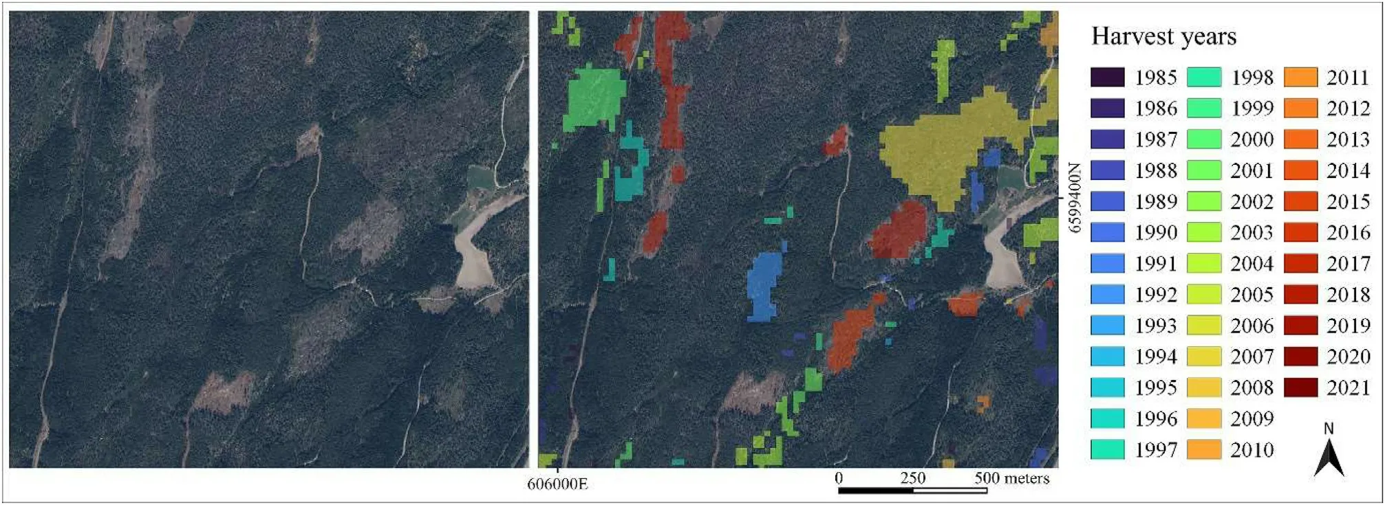
Fig.4.Map of harvested areas in southeastern Norway.

The definition of near-natural forests is based on the concept of biologically old forests, as described by Søgaard et al.(2012).In this study, a forest stand is considered near-natural if its age exceeds the harvest maturity age.We used the maturity age criteria defined by the Norwegian NFI (Viken, 2018), which is founded on the H40 site index system.The minimum threshold for determining a stand as old is defined based on site productivity and dominant tree species (Table 1).Plots located in stands older than the minimum threshold were defined as near-natural forests, whereas plots in younger stands were defined as managed forests.

The definition of semi-natural forests used in this study follows the criteria established by Storaunet and Rolstad (2015).According to this definition,mature forest stands that were classified as development class V at the time of the establishment of the permanent plots between 1986 and 1993 and remained classified as development class V during the most recent forest inventory, are considered semi-natural forests.However,information regarding the development class of permanent plots in protected areas and additional plots in old forests is not available for this period.To overcome this limitation, the development class was retroactively determined for 1995 for all datasets.It was determined based on the site index,age,and species of the two largest trees for the additional plots in old forests, and the dominant species, stand age, and the site index registered during the latest inventory for the permanent plots and the permanent plots in protected areas.See supplementary materials for an error assessment of the development class determined for the last forest inventory(Table S1)and for 1995(Table S2).Photos of managed,semi-natural,near-natural,and pristine forests were presented in Fig.2.

Table 2 summarized the number of permanent plots,permanent plots in protected areas,and additional plots in old forests for each of the three natural forest definitions and stratified by dominant tree species.The three definitions of natural forests,i.e.,pristine,near-natural,and seminatural, were not mutually exclusive (Fig.3).A forest may possess characteristics that align with more than one definition, depending on factors such as its age, management history, and ecological context.Consequently,some plots can be classified as pristine,near-natural,and semi-natural forests simultaneously.Across all datasets, a larger percentage of plots were defined as semi-natural forests(24%),followed by pristine(10%)and near-natural forests(6%).Regardless of the definition used, a larger percentage of the additional plots in old forests were defined as natural forests compared to the permanent plots and the permanent plots in protected areas.Specifically,65%of additional plots in old forests were defined as pristine forests, while only 3% of permanent plots fell under this class.Furthermore, around 90% of the plots defined as near-natural forests were also defined as semi-natural forests.Of the total number of plots defined,4%,9%,and 10%were considered natural forests by the three definitions for the permanent plots, the permanent plots in protected areas,and the additional plots in old forests,respectively.

2.4.Remotely sensed data

2.4.1.ALS data and derived products

The study utilized ALS data downloaded from the website: hoydedata.no.The point clouds were recorded across 104 different acquisition projects between 2007 and 2020 and were downloaded in 2020.The point density ranged from 0.5 to 10 points·m-2.When multiple ALS datasets covered a plot,the most recent project was selected for analysis.The maximum time gap between the ALS data acquisition and the field data collection was ten years for two plots,while 98%of the plots had a time gap of ≤5 years.Additionally, ALS-derived digital terrain models(DTM) at a spatial resolution of 1 and 10 m and ALS-derived digital surface models (DSM) at a spatial resolution of 1 m were downloaded from the same website in 2022.The DTMs were produced by triangulation with natural neighbor interpolation of the ground ALS points,while the DSMs were constructed by assigning the maximum value to each bin.These models were generated from a mosaic of the most recent ALS data collected from 2007 to 2022.To create canopy height models(CHM),the DTM at a spatial resolution of 1 m was subtracted from the DSM.Pixels with a height ＜3 m were removed from the CHMs to identify gaps in the canopy,and a sieve filter with five pixels including eight connectedness was used to remove gaps smaller than 5 m2(Vehmas et al., 2011;Vepakomma et al., 2008).Trees were identified on the CHMs using a local maximum filter with a window size of 3 m in diameter, and those with height ＞50 m or ＜2 m were excluded.Finally, individual crowns were delineated using a region-growing algorithm (Dalponte and Coomes, 2016) based on the identified trees’ locations, and the maximum crown size was set to 3 m.

2.4.2.Map of change

To produce a map of harvested areas, LandTrendr, a temporal segmentation algorithm implemented on Google Earth Engine (Kennedy et al., 2010), was used.The algorithm identifies short-duration events and long-term trends in time-series made up of yearly image composites from Landsat-5 TM, Landsat-7 ETM+, and Landsat-8 OLI.In this study,the algorithm was run for images acquired during the growing season in Norway (from June to September) between 1985 and 2021, using the normalized burnt ratio index generated from near-infrared and Short-Wave Infrared 2 bands to create the image composite.The default control parameter values defined in Kennedy et al.(2018)were used.See supplementary materials for a full description of the LandTrendr parameters used to produce the map of harvested areas (Table S3).To eliminate noise,a sieve filter of four pixels including eight connectedness was applied.The procedure is fully described in Jutras-Perreault et al.(2021).The year of harvest, if any, was extracted at the center of each plot.A map of harvested areas was presented in Fig.4.

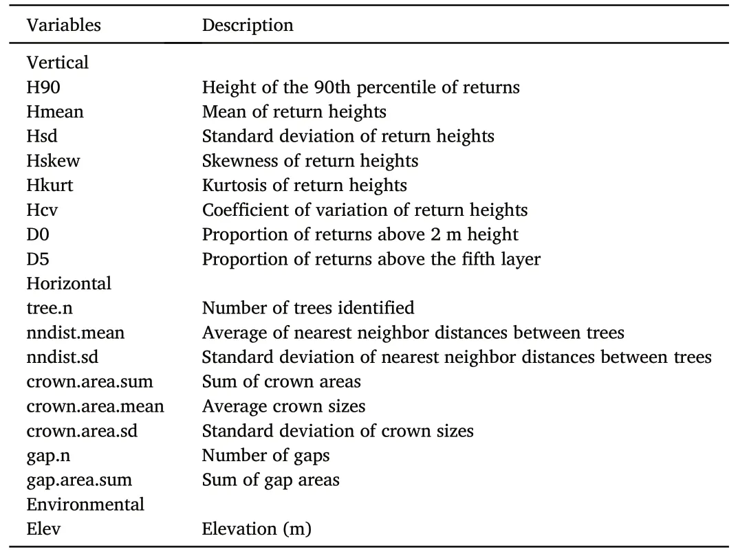
Table 3ALS variables analyzed to predict the presence of natural forests.

The plot locations were verified against the map of change.If a harvesting event was identified prior to the acquisition of the field data,plots originally classified as semi-natural or near-natural forests were redefined as managed forests.However, this adjustment was not applied to pristine forests, as forest management activity for this definition was assessed through on-site visual evaluation.

2.4.3.Variables

Vertical variables derived from ALS data provide information about the vertical distribution of the forest canopy cover.They were computed for each sample plot following the procedure described in Næsset(2004)from the relative height of all first returns ＞2 m.The relative height was calculated from the difference between the return height value and the terrain height.The ALS variables included height metrics based on the 10th, 20th, …, 90thpercentile (H10, H20, …, H90), the mean (Hmean),standard deviation (Hsd), skewness (Hskew), kurtosis (Hkurt), and coefficient of variation (Hcv), and density metrics calculated from the proportion of returns above 10 vertical layers to the total number of returns(D0,D1,…,D9).The layers were of equal height,i.e.,one-tenth of the height range between the 2 m threshold and the 95thpercentile(H95).From these variables,only Hmean,Hsd,Hcv,Hkurt,Hskew,H90,D0,and D5 were retained for analysis since successive height and density metrics based on ALS data are highly correlated.

Horizontal variables were computed for each plot from the location and the size of the identified trees and gaps.These variables include the number of trees (tree.n), the average and standard deviation of the nearest neighbor distances (nndist.mean, nndist.sd), the sum of the crown area (crown.area.sum), the average crown size (crown.area.mean),and the standard deviation of the crown size(crown.area.sd).Additionally,we summed the number of gaps(gap.n)and their total area(gap.area.sum) per plot.To compute these horizontal variables, a minimum of two identified trees per plot was required.As a result, the horizontal variables could not be computed for 55 permanent plots, one permanent plot in protected areas,and one additional plot in old forests.

The elevation at the center of each plot was obtained from the 10 m resolution DTM.An overview of the variables that were analyzed for their potential to predict the presence of natural forests is presented in Table 3.

2.5.Statistical models

We used GLM models with a binomial logit link function to predict the presence of pristine, near-natural, and semi-natural forests.Models were built for a total of four combinations using the field data from the permanent plots only or in combination with the permanent plots in protected areas and/or the additional plots in old forests (Fig.5).The models were applied separately to each species stratum,i.e.,spruce,pine,or mixed, as well as to the unstratified data.We constructed three variations of the models:using all variables,only vertical variables,and only horizontal variables.A best subset model selection based on Akaike information criterion(AIC)was used to identify up to three variables.The limitation to three variables was implemented to avoid overfitting the models to specific datasets and prioritize the depiction of overall trends.Models with multicollinearity, i.e., with a variance inflation factor exceeding five, were excluded.Given the low occurrence of natural forests in the field data,we used both balanced and original datasets for the analysis.To ensure equal representation of both presence and absence of natural forests,we oversampled the minority class and undersampled the majority class.Random observations were selected from the majority class and removed.To oversample the minority class,we used a synthetic minority oversampling technique (Chawla et al., 2002) to generate a large population of observations, from which observations were randomly selected.Synthetic observations were created using k-nearest neighbors on the minority class.

Each model was validated using field data from the permanent plots,permanent plots in protected areas, and additional plots in old forests.For models constructed using the same dataset as the validation,either 5-fold cross validation (5-fold CV) or leave-one-out cross validation(LOOCV)was employed.Specifically,5-fold CV was used for models built using the permanent plots,except for pine-stratified data where LOOCV was used instead.LOOCV was therefore chosen in cases where there were insufficient observations in the minority class to perform a 5-fold CV.To ensure that predictions were not validated against synthetic observations, field datasets used for both model construction and validation predictions were not balanced.

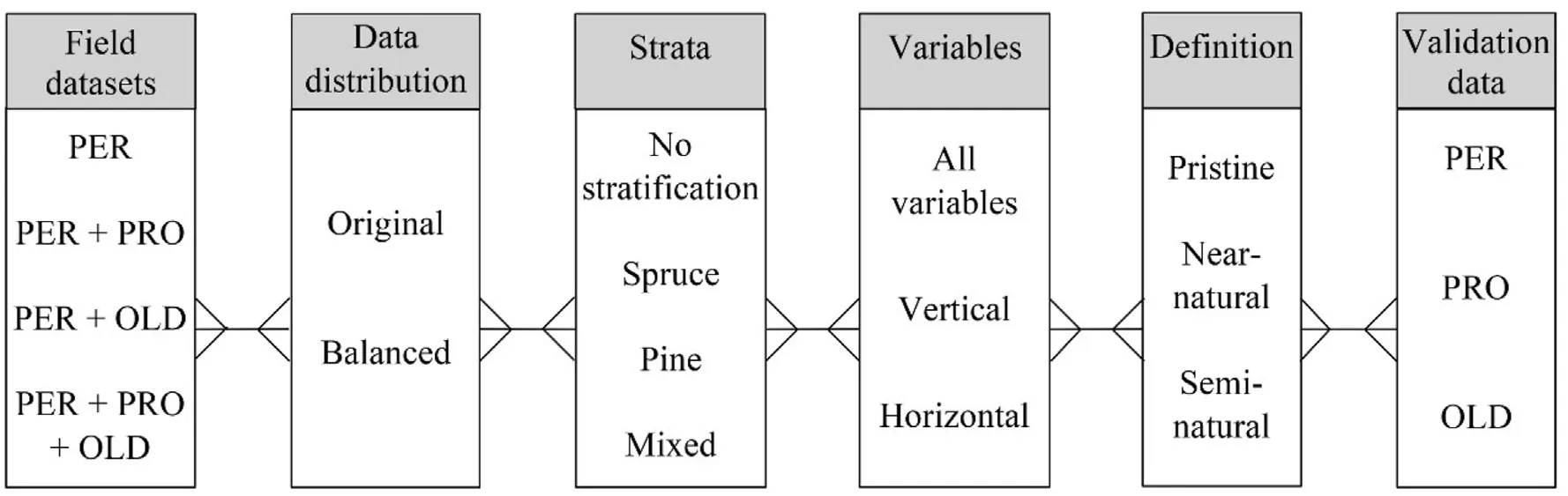
Fig.5.Flow chart illustrating the different combinations of field datasets,including permanent plots(PER),permanent plots in protected area(PRO),and additional plots in old forests(OLD),along with ALS-derived variables for predicting the presence of pristine,near-natural,and semi-natural forests.The field datasets were used in both their original distribution and balanced forms,and the plots were stratified based on the dominant tree species.The predictions obtained were validated using the PER, PRO, and OLD datasets.

Fig.6.Map of natural forests in southeastern Norway.

The contribution of each variable in constructing the models was evaluated by counting the number of times they were selected.For each model, the variables selected were recorded at each fold, and the proportion of the time each variable was selected was reported.

We evaluated the performance of the models using precision, recall,and Matthew's correlation coefficient(MCC),which were calculated from the confusion matrix.Precision measures the proportion of true positives out of all positive predictions, while recall measures the proportion of true positives out of all actual positives.MCC quantifies the agreement between actual and predicted values of a binary classification.It produces a high score only if the predictions perform well for all four quadrants of the confusion matrix, making it a more reliable measure than Kappa and F1 score for unbalanced datasets (Chicco and Jurman,2020).Values of MCC ranges from -1 to 1, with a perfect prediction resulting in a score of 1 and perfect disagreement resulting in a score of-1.A value close to 0 indicates that the model performs similar to what could be expected under randomness(Baldi et al.,2000).MCC was also used to assess the potential gain resulting from the incorporation of additional data and through data stratification by dominant tree species.

To compute the confusion matrices,we determined the best threshold point based on the MCC-F1 curve.The MCC-F1 curve incorporated two metrics, MCC and F1 score, which summarized the performance of the entire confusion matrix by including all four quadrants.Cao et al.(2020)showed that this approach effectively distinguished between good and bad classifiers in imbalanced datasets.The threshold point on the MCC-F1 curve that resulted in the closest value to perfect performance,i.e.,MCC and F1 both equal to 1,was considered the best.

2.6.Analysis

The accuracy of the models’predictions was assessed for each natural forest definition, considering different combinations of datasets used to build the models and to perform predictions.The assessment was performed for both balanced and original datasets, as well as for stratified data.Finally,the study identified the most frequently selected variables used in building the models, and a comparison was performed between the performance of the vertical and horizontal variables to predict the presence of natural forests.

3.Results

A map of pristine,near-natural,and semi-natural forests for an area of approximately 10 km2southeast of Oslo is presented in Fig.6.

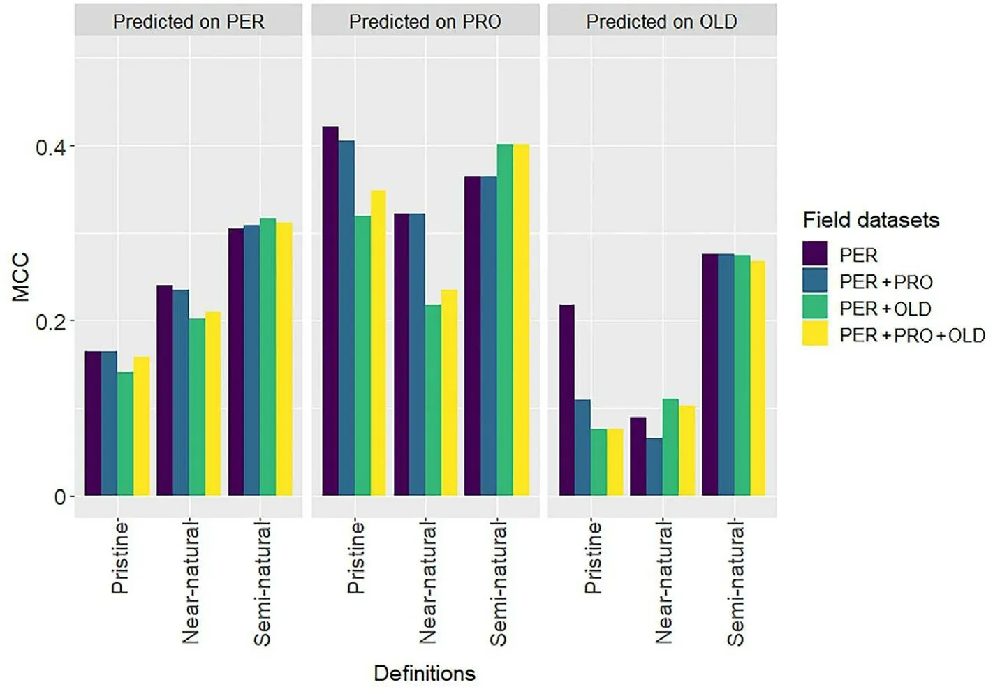
Fig.7.Models'performance in predicting the presence of pristine,near-natural,and semi-natural forests.The predictions were performed on permanent plots(PER),on permanent plots in protected areas (PRO), and on additional plots in old forests (OLD) using different combination of field data.MCC: Matthew's correlation coefficient.See supplementary materials for detailed statistical analysis (Table S4).

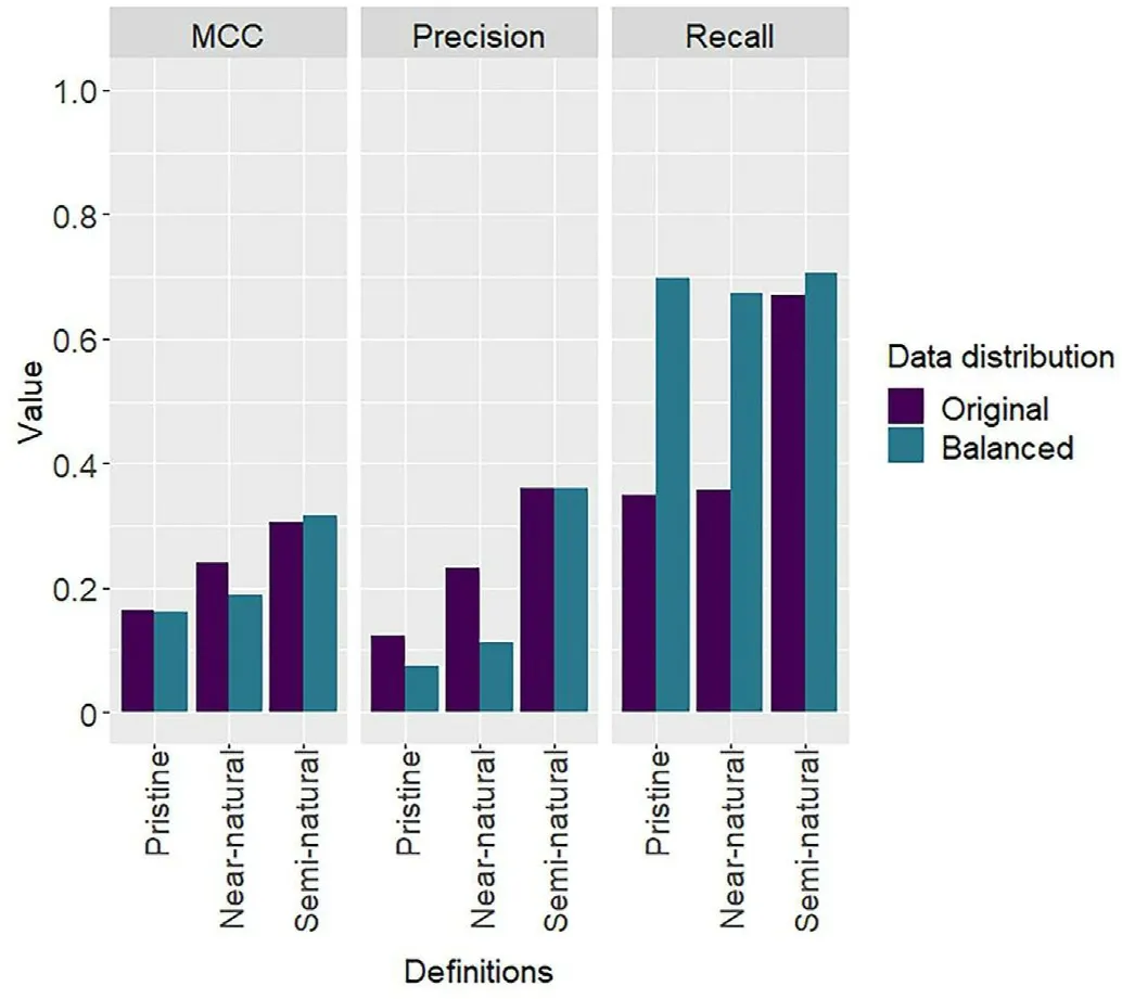
Fig.8.Models'performance in predicting the presence of pristine,near-natural,and semi-natural forests using the original and balanced distributions of the permanent plots.MCC: Matthew's correlation coefficient.See supplementary materials for detailed statistical analysis (Table S5).

The most accurate predictions, regardless of the natural definition applied or the combination of field data used to build the models, were obtained when predicting on the permanent plots in protected areas(Fig.7).The maximum MCC values achieved for pristine, near-natural,and semi-natural forests were 0.42, 0.32, and 0.40, respectively.In contrast, when predicting on additional plots in old forests, maximum MCC values were smaller,reaching 0.22,0.11 and 0.28 for pristine,nearnatural, and semi-natural forests, respectively.When predicting on permanent plots, maximum MCC values of 0.17, 0.24, and 0.32 were obtained for pristine, near-natural, and semi-natural forests, respectively.Combining the permanent plots,permanent plots in protected areas,and the additional plots in old forests did not substantially improve the predictions for the three definitions.

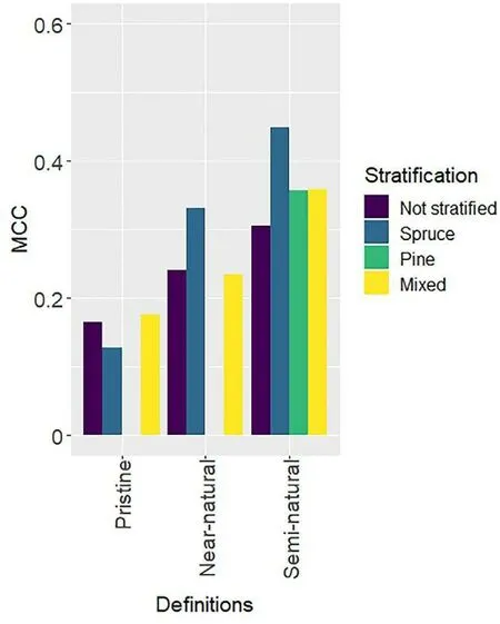
Fig.9.Models'performance in predicting the presence of pristine,near-natural,and semi-natural forests using permanent plots stratified per dominant tree species and unstratified.MCC: Matthew's correlation coefficient.See supplementary materials for detailed statistical analysis (Table S6).

Balancing the field data did not improve the predictions(Fig.8).The use of balanced datasets resulted in larger recall values but smaller precision values for pristine and near-natural forests, indicating a smaller omission error at the expense of a larger commission error.

Fig.10.Variable importance for the prediction of pristine, near-natural, and semi-natural forests for models built with permanent plots.Hmean, Hsd, Hcv, Hkurt,Hskew, H90, are the mean, standard deviation (sd), coefficient of variation, kurtosis, skewness, and 90th percentile of return heights, respectively; D0 and D5:proportion of return above 2 m height and proportion of returns above the 5th layer;tree.n: number of trees identified;nndist.mean and nndist.sd:average and sd of nearest neighbor distances between trees;crown.area.sum:sum of crown areas;crown.area.mean and crown.area.sd:average and sd of crown sizes;gap.n:number of gaps; gap.area.sum: sum of gap areas; Elev: elevation.

Stratifying the plots based on the dominant tree species had varying impacts on the predictive power of the models depending on the definition of natural forest used (Fig.9).Since there were not enough plots classified as pristine and near-natural forests dominated by pines, a stratification based on pine was not possible for these two definitions.Better predictions of pristine forests were achieved using unstratified data,while the stratification by species improved the predictions of nearnatural and semi-natural forests.An increase in MCC values of 0.09 was observed for the spruce stratum when predicting the presence of nearnatural forests.The prediction of semi-natural forests was improved regardless of the stratum used, with an increase in MCC values of 0.15,0.05,and 0.05 for spruce,pine,and mixed strata,respectively.

The variable Elev was systematically selected when developing predictive models using permanent plots for all three definitions (Fig.10).The second most frequently selected variable was Hsd,which proved to be important for the unstratified data and the spruce stratum.Additionally, when considering the reference data stratified by spruce,crown.area.mean emerged as an important variable for all definitions.On average, the permanent plots classified as natural forests were found to be located at elevations approximately 230, 80, and 40 m higher than those classified as managed forests for the definitions of pristine, nearnatural, and semi-natural forests, respectively.Furthermore, regardless of the definition used, the average values of Hsd, crown.area.mean, D0,and D5 were consistently larger in natural forests compared to managed forests.The use of horizontal variables did not substantially improve the predictions(Fig.11).

4.Discussion

The vertical distribution of the biological material varies among managed, semi-natural, and pristine forests, and this distinction can be reflected in the vertical distribution of the ALS point clouds(Fig.12).In managed forests, ALS returns predominantly occur within the canopy,whereas in pristine forests, the returns are distributed throughout the entire height profile.This variation can be attributed to the more complex vertical structure and the presence of canopy gaps in pristine forests,allowing ALS measurements to capture a wider range of heights.

4.1.Error sources

The smaller predictive accuracy of near-natural or pristine forests compared to semi-natural forests may be attributed to the smaller proportion of observations in the minority class.Additionally,the nonlinear relationships between the stand age and height make it challenging to accurately predict age with ALS data.This is reflected in the smaller precision values for near-natural forests, which have a larger age threshold than semi-natural forests, resulting in confusion between younger and older forests of similar heights.Pristine forests exhibit greater variation in the spatial distribution of the trees,which is not wellcaptured by standard area-based ALS metrics.This larger horizontal complexity is supported by the selection of nndist.sd and crown.mean.area,two horizontal variables,as among the most important variables for predicting pristine forests.Moreover,the classification of a forest as pristine is more subjective and may therefore be subject to systematic misclassification by the field workers.

The definitions of near-natural and semi-natural forests are based on the site index of the stand.The calculation of a stand's site index is based on the species,age,and height of two large dominant trees present in the stand, selected through visual assessment, which is prone to variation between forest inventory workers.Consequently, discrepancies in the tree selection can lead to differences in the site index, affecting the classification of the stand as near-natural or managed forest.Underestimating the site index can increase the lower age threshold required to classify a stand as near-natural forests, resulting in misclassification.Furthermore,site index,along with the age and species of two dominant trees, is used to determine the development class of a stand.Inaccurate site index or variations in the tree selection can influence the development class estimation,which in turn can result in misclassification of the plots as semi-natural or managed forests.Moreover,retroactively calculating the development class based on the assumption that the same trees would have been selected in both the most recent inventory campaign and in 1995 can introduce errors since different trees may have been selected based on the stand's characteristics at the time.Furthermore,although site index is typically assumed to remain constant for a specific stand over time, research has shown that it can vary (Bontemps et al.,2009;Socha et al.,2021).Several factors,such as increasing atmospheric nitrogen deposition and climate change, have been identified as contributors to this variability (Ågren et al., 2008).Additionally, site index systems such as the H40 system assume that the forest is even-aged(Tveite, 1977).However, this assumption is frequently violated in various types of inventories,and it is particularly prone to violation when determining the site index of natural forests, as they are commonly characterized by uneven-aged stands.

The map of change was utilized to identify plots classified as nearnatural or semi-natural forests that had undergone harvest operations.They were subsequently classified as managed forests, as they did not meet the requirements for natural forests.However,it is possible that the detection of a change could have been triggered by natural disturbances,such as windthrow, leading to the incorrect classification of a plots.To improve the accuracy of change detection,it may be necessary to adjust the various parameters used, such as the duration of a disturbance, to better account for regional conditions.

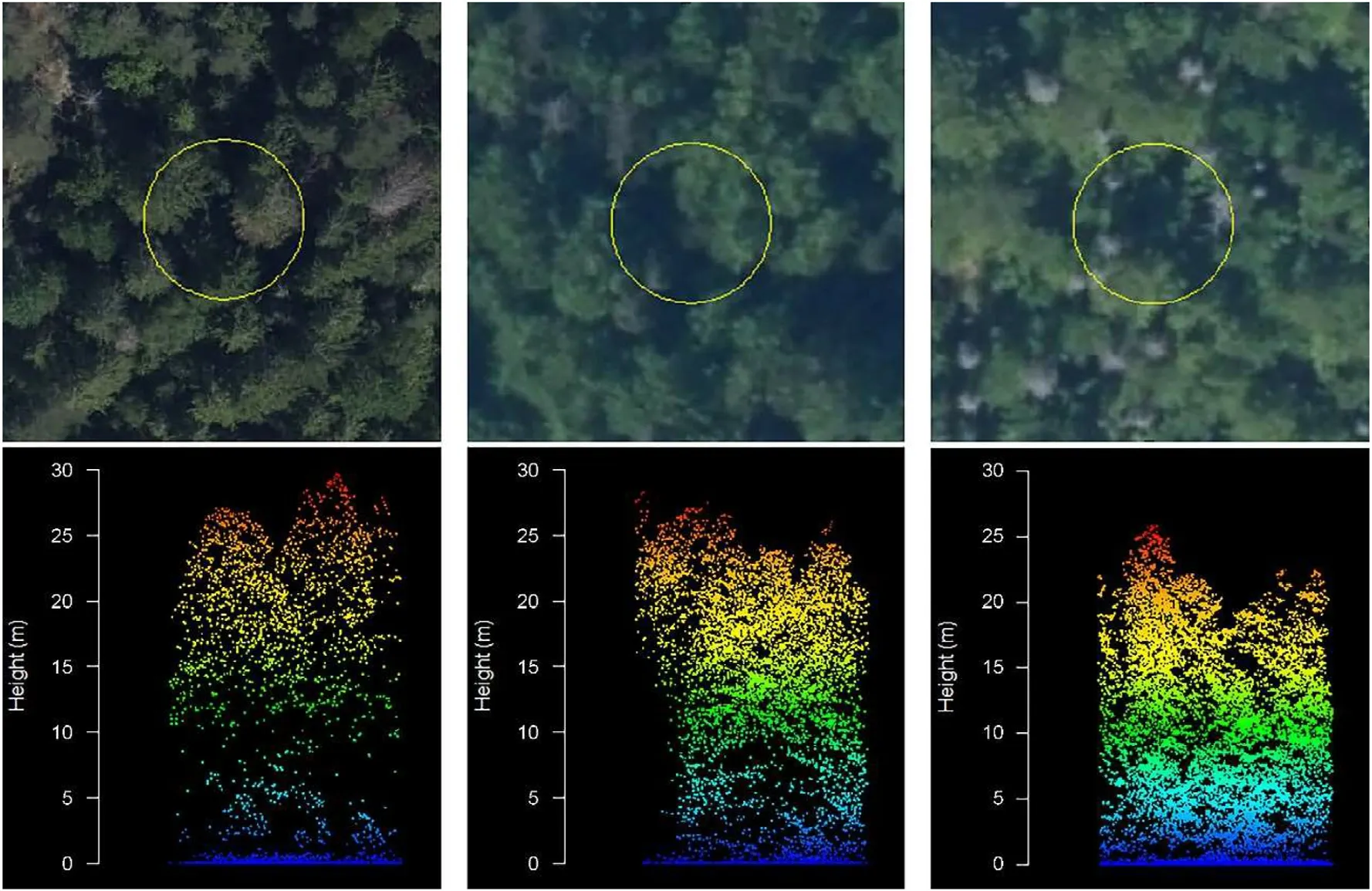
Fig.12.Vertical distribution of ALS point clouds within plots in managed (left), semi-natural (center), and pristine (right) forests.

When using ALS data acquired from different projects at different times, several challenges arise.The time delay between the ALS acquisition and the inventory campaign can vary considerably across regions,as can the sensor properties, including point density and scan angle.These variations can introduce discrepancies in the accuracy of the ALSderived metrics, making it difficult to compare and combine data from the different acquisition projects.Although incorporating the ALS project as a random variable in predictive models could account for some of the differences(Ørka et al.,2022),there may not be sufficient natural forest plots available per project to accomplish this in certain cases.

4.2.Stratification and additional field data

The stratification of field data based on the dominant tree species,particularly for plots dominated by spruce, had a positive impact on predictions.However, the number of pine-dominated plots was insufficient to construct predictive models specifically for a pine-dominated stratum, except when predicting semi-natural forests.To increase the representation of observed plots with natural forests, additional plots were sampled within old forest stands based on existing mapping of old high conservation value forests.However, neither the inclusion of additional plots nor balancing the dataset improved the predictions.The distribution of these additional plots was most likely prone to systematic errors as the plots were subjectively selected within the same stratum.The plots lacked sufficient variation among them and likely fell within a range where the model's prediction accuracy was already good.In the case of unbalanced datasets, using the MCC-F1 curve to determine the threshold yielded good results without the need for generating synthetic observations.Introducing synthetic observations resulted in commission errors when predicting pristine and near-natural forests.

4.3.Variables

Our results diverge from those of Sverdrup-Thygeson et al.(2016)regarding the relative importance and significance of vertical and horizontal variables in distinguishing between natural and managed forests.While their study found that horizontal variables outperformed vertical variables,our analysis showed that vertical variables were more effective and were selected more frequently in predictive models.We propose two possible explanations for this discrepancy.First,Sverdrup-Thygeson et al.(2016) used field data consisting of 0.2 ha plots,while we used 250 m2plots.The smaller plot size in our study failed to capture the horizontal variation within each plot, which have affected the accuracy of the horizontal variables.Second,the horizontal metrics were computed from CHMs constructed using a mosaic of ALS data collected from 2007 to 2022, whereas the vertical metrics were derived from ALS point clouds collected between 2007 and 2020.Consequently, the computation of horizontal variables incorporated more recent ALS acquisition, which may have introduced potential discrepancy between the status of the plots as depicted by the vertical variables compared to the horizontal variables.

4.4.Further work

To capture different degrees of naturalness, we employed three distinct definitions of natural forests, ranging from pristine forests representing the highest level to semi-natural forests representing a lower level of naturalness.However, to further improve these definitions, or develop new and more comprehensive ones, additional factors such as proximity to forest roads, slope, presence of old forests, deadwood, and forest connectivity could be taken into consideration.A multi-criteria analysis that incorporates the likelihood of human intervention and the significance of biophysical properties of forests could also be utilized to create indices of naturalness.Similar indices have already been developed by other researchers, such as Potapov et al.(2008) and Svensson et al.(2020).

5.Conclusion

Our study highlights the significance of ALS data for natural forest detection.The vertical distribution of the ALS point cloud offers valuable insights into the natural character of forest cover.Given the importance of natural forests in maintaining biodiversity, it is essential to protect areas with high conservation value.Our findings provide valuable guidance for decision-making processes aimed at increasing the proportion of forested areas that are protected.Using ALS data,we predicted the presence of natural forests according to three definitions.We found that stratifying the data by species improved the accuracy of our predictions,whereas acquiring additional field data targeting natural forests for better balance in the dataset did not yield significant improvements.Accurately identifying the location of natural forests is crucial for making informed decisions about which areas to preserve.Our study provides a foundation for further research on the use of ALS data for the detection and conservation of natural forests.

Funding

The study received funding under the umbrella of ERA-NET Cofund ForestValue project NOBEL,“Novel business models and mechanisms for the sustainable supply of and payment for forest ecosystem services”.ForestValue was funded by the European Union's Horizon 2020 research and innovation program (grant number 773324).Furthermore, the Norwegian Environment Agency funded the collection of the additional plots as a part of the project “Remote sensing-based mapping and monitoring of the forest ecosystem” (grant number 18087221).This study was also supported by the Norwegian Research Council (project number 297883).

Authors’contribution

Conceptualization, M.C.J.P., T.G., E.N.and H.O.Ø.; methodology,M.C.J.P.and H.O.Ø.; formal analysis, M.C.J.P.and H.O.Ø.; writing -original draft preparation, M.C.J.P.; writing - review and editing,M.C.J.P., T.G., E.N.and H.O.Ø.; visualization, M.C.J.P.; project administration,T.G.and H.O.Ø.;funding acquisition,T.G.,E.N.and H.O.Ø.All authors reviewed the results and approved the final version of the manuscript.

Declaration of competing interest

The authors declare that they have no known competing financial interests or personal relationships that could have appeared to influence the work reported in this paper.

Acknowledgements

The authors would like to thank Dr.Marius Hauglin from the Norwegian Institute of Bioeconomy Research for providing the NFI data and Mr.Jaime Candelas Bielza, Norwegian University of Life Sciences, for processing the ALS data, and the administrative authorities in nature conservation areas for permission to do tree coring.

Appendix A.Supplementary data

Supplementary data to this article can be found online at https://doi.i.org/10.1016/j.fecs.2023.100146.