Nonlinear direct data-driven control for UAV formation flight system

WANG Jianhong, Ricardo A. RAMIREZ-MENDOZA, and XU Yang

1.School of Engineering and Sciences, Tecnologico de Monterrey, Monterrey 64849, Mexico;2.School of Civil Aviation, Northwestern Polytechnical University, Xi’an 710072, China

Abstract: This paper proposes the nonlinear direct data-driven control from theoretical analysis and practical engineering, i.e.,unmanned aerial vehicle (UAV) formation flight system.Firstly,from the theoretical point of view, consider one nonlinear closedloop system with a nonlinear plant and nonlinear feed-forward controller simultaneously.To avoid the complex identification process for that nonlinear plant, a nonlinear direct data-driven control strategy is proposed to design that nonlinear feed-forward controller only through the input-output measured data sequence directly, whose detailed explicit forms are model inverse method and approximated analysis method.Secondly,from the practical point of view, after reviewing the UAV formation flight system, nonlinear direct data-driven control is applied in designing the formation controller, so that the followers can track the leader’s desired trajectory during one small time instant only through solving one data fitting problem.Since most natural phenomena have nonlinear properties, the direct method must be the better one.Corresponding system identification and control algorithms are required to be proposed for those nonlinear systems, and the direct nonlinear controller design is the purpose of this paper.

Keywords: nonlinear system, nonlinear direct data-driven control, model inverse control, unmanned aerial vehicle (UAV) formation flight.

1.Introduction

Automatic control theory is the area of application-oriented mathematics that deals with the basic principles underlying the analysis and design of control systems.To control an object means to influence its behavior so as to achieve a desired goal.In order to implement this influence, engineers build devices that incorporate various mathematical techniques.These devices range from Watt’s steam engine governor, designed during the English Industrial Revolution, to the sophisticated microprocessor controllers found in consumer items, such as industrial robots, airplane autopilots, and unmanned aerial vehicles (UAVs) [1].The study of these devices and their interaction with the object being controlled is the subject of automatic control theory.While on the one hand, one wants to understand the fundamental limitations that mathematics imposes on what is achievable, irrespective of the precise technology being used, it is also true that technology may well influence the type of question to be asked and the choice of mathematical model [2].

Roughly speaking, there have been two main lines of work in automatic control theory, which sometimes seem to proceed in very different directions but are in fact complementary [3].One of these is based on the idea that a good model of the object to be controlled is available and that one wants to somehow optimize its behavior.For instance, physical principles and engineering specifications can be used in order to calculate the trajectory of a spacecraft which minimizes total travel time or fuel consumption.Sometimes, the use of feedback is considered to correct for deviations from the desired behavior.For instance, various feedback control systems are used during actual space flight to compensate for errors from the precomputed trajectory.

The above-described control strategy based on one good model of the considered plant is called model-based control, has existed for many years, and it has been studied from theory and engineering practice since the 1930s.On the contrary, a new concept of science has appeared in recent years [4], i.e., lots of data are collected through some advanced sensors or physical devices, then the goal of this paper is to extract that important useful information from these interesting data sets or sequence by virtue of some statistical or other mathematical tools in [5], such as machine learning, reinforcement learning, and deep learning.For example, system identification is to construct one mathematical model for the unknown plant from the collected input-output data sequence, then this constructed mathematical model is beneficial for the latter controller design or other interesting considerations.Due to the physical principle for system identification,i.e., information about the unknown plant belongs to the data, similar information about the unknown controller is also included in the data [6].Then the goal of this paper is to modify or design the unknown controller from data too, while not identifying the unknown plant, i.e., direct data-driven control.

Compared model-based control with direct data-driven control, model-based control needs two steps, i.e., identification, and control.But direct data-driven control designs the unknown controller directly from the collected input-output data sequence, i.e., only one step is needed in designing the unknown controller while avoiding that different system identification process [7].Also,the above description is the reason why direct data-driven control is more widely studied all over the country.

As the number of references about direct data-driven control is vast, but only the ones related to our work about nonlinear direct data-driven control.To the best of the authors’ knowledge, all theories about linear cases are very mature.Our ongoing missions are concentrated on nonlinear cases, i.e., nonlinear system identification, nonlinear controller design, nonlinear analysis, etc., as during the living situation, all physical phenomena are nonlinear.It means linear system theory is an ideal case, but it is not suited for the real system.Therefore, it is very urgent to extend the existing research on nonlinear direct data-driven control.Milanese et al.proposed a set membership prediction for a nonlinear system with unknown but bounded noise [8].This output prediction was not a constant value, but a guaranteed interval with the desired probabilistic level [9].After obtaining this output prediction and substituting it into one regularized cost function,the direct data direct driven predictive control was yielded.The novel adaptation was combined with direct data-driven control to form adaptive receding horizon control [10], which proves its efficient application in designing one industrial controller.An online direct approach was introduced into direct data-driven control for nonlinear systems [11], where a recursive identification strategy was applied to modify the unknown controller parameter iteratively.Some other aspects or properties were analyzed in learning a nonlinear controller from data, for example, theory, computation, and experimental results [12].The guaranteed simulation accuracy for output prediction was done in [13], where the asymptotic results were appropriate for a linear system, not for the nonlinear system.The above-mentioned references are related to nonlinear system identification, i.e., using the collected input-output data sequence to identify that unknown plant.But all of the above results can be applied to nonlinear controller design by using direct data-driven,i.e., nonlinear direct data-driven control.

During these two years, our team also made some new contributions to direct data-driven control.More specifically, stability analysis was given for nonlinear closedloop systems with nonlinear systems and nonlinear controllers simultaneously [14].A novel direct data-driven strategy was proposed for linear parameter-varying closed-loop systems in [15], where system identification,numerical optimization, power spectral, and optimal input design were all combined within the proposed general framework.In [16], this direct data-driven model reference control framework was presented for the flight simulation table, and its corresponding synthesis analysis was seen in [17], such as persistent excitation, optimal state feedback controller, output predictor, and stability.Wang et al.connected adaptive control and direct datadriven control to adjust the controller parameters adaptively for one closed-loop system.Generally, the previous contributions to direct data-driven control are mainly for linear systems, and few for nonlinear systems [18].Zeilinger et al.combined deep learning and robust model predictive control to consider some uncertain factors,existing in engineering [19].If the output of aircraft is restricted into one limited range, denoted as one tube,then the tube model predictive control was applied to get the limited output response [20].Furthermore, UAV formation flight control is equivalent to a multi-agent control problem in [21-23], where all the elements of all the agent states reach consensus at the same time, i.e., the multi-agent system achieves time-synchronized consensus and fixed-time-synchronized consensus.

Based on the above-mentioned references and our previous contributions to direct data-driven control, this paper is concerned with nonlinear direct data-driven control from theory and its application in UAV formation flight systems.From the theoretical perspective, consider one closed-loop nonlinear system structure with one nonlinear plant and one nonlinear controller simultaneously,the mission of nonlinear direct data-driven control is to design that nonlinear controller only through collecting input-output data sequence while avoiding the identification process for that nonlinear plant.After reviewing the model inverse method for designing a nonlinear controller, we propose an approximated analysis method to give a detailed form for the nonlinear controller.Generally, the model inverse method holds for the case of white noise, and to use one linear controller to replace the nonlinear controller, the approximated analysis method is applied to drive some necessary and sufficient conditions,which guarantee the approximated property, i.e., the nonlinear output is same with the approximated linear output.From an applied point of view, all theoretical results are proven efficient in UAV formation flight systems.After introducing the UAV formation flight system in detail,one closed-loop nonlinear system structure is reformulated to be similar to the considered system structure.Then the considered nonlinear direct data-driven control is proposed to design the flight controller, while satisfying some important performances, for example, stability and tracking.

In summary, two new contributions of this paper are formulated as follows.

(i) Nonlinear direct data-driven control is applied to design the nonlinear controller.

(ii) The detailed process of applying nonlinear direct data-driven control into UAV formation flight systems is given so that our ongoing work combines theoretical research and engineering application.

This paper is organized as follows.In Section 2, the considered closed-loop system with one nonlinear plant and nonlinear controller is presented.To design this nonlinear controller without any information about nonlinear plants, a nonlinear direct data-driven control is proposed to be two different forms, corresponding to two cases,i.e., model inverse method and approximated analysis method in Section 3.Section 4 introduces the basic prior knowledge of the UAV formation flight system, then one special flight system structure is reformulated.Section 5 gives some numerical examples to testify to the studied nonlinear direct data-driven control from an applied point of view.Section 6 formulates the main conclusion and points out the future work.Roughly speaking, this paper is divided into two parts, which study nonlinear direct data-driven control from theory and application respectively.

2.Nonlinear system structure

Consider a closed-loop system with a nonlinear plant and nonlinear feed-forward controller, i.e., unit feedback, as shown in Fig.1.

In Fig.1,K(·) is one nonlinear feed-forward control,f(·)is one nonlinear plant or system, and they are also unknown.r(t) is the external input signal, corresponding to the whole closed-loop system.u(t) is one input signal for the nonlinear plantf(·).y(t) is the output signal for the whole closed-loop system.External noisee(t) is added in the outputy(t).Error signal ε(t) embodies the essence of unit feedback, i.e.,

wheretis the time variable.

As nonlinear plantf(·) and nonlinear feed-forward controllerK(·) are considered here, they cannot expand to their linear parameterized forms respectively.From Fig.1, the following nonlinear relations hold

Then, the outputy(t)is rewritten as

Combining the above nonlinear system description and nonlinear relations (1) and (2), our mission is to construct nonlinear feed-forward controllerK(·), while avoiding the nonlinear system identification process for that nonlinear plantf(·).

3.Nonlinear direct data-driven control

Although the nonlinear plantf(·) is unknown, its inputoutput data are collected to form one data set, i.e.,{u(t),y(t)}, whereNis the total number of data.Given that external input signalr(t) , an error signal ε(t)=r(t)-y(t)is yielded, so the input-output data set

is also obtained for the nonlinear feed-forward controllerK(·).More generally, the proposed direct data-driven control is to design a nonlinear feed-forward controllerK(·)based on this input-output data set:

The detailed nonlinear controller design processes are formulated as following three subsections.

3.1 Model inverse method

That nonlinear feed-forward controllerK(·) can be generated by the model inverse method directly, as the output signalu(t), corresponding to the nonlinear feed-forward controllerK(·), is collected online.Its inverse relation is used to design the output signalu(t) through the following optimization problem, i.e.,

where two regularized constants ρyand ρuare defined as follows

where notation //·// is the commonly used Euclidean norm.

The parameter µ>0 is chosen by designers and trades off the tracking accuracy and computational complexity.From (3) and (4), the first step for the model inverse method is to collect three kinds of signals, i.e.,{r(t),u(t),y(t)}, the nonlinear controller is generated through one numerical optimization problem.Then the ideal case satisfies thatr(t)=y(t), i.e.,

Generally, the model inverse method is reformulated as follows.

Step 1 Collect some signals to form a data set:

Step 2 Use that numerical optimization problem to yield one optimal nonlinear controller.

Step 3 Check whether the error signal is zero, i.e.,

If ε(t)=r(t)-y(t)=0, then accept that obtain nonlinear controller, or apply a new inputr(t) to excite that closed-loop system and repeat the above steps, until that error signal ε(t) is zero, then terminate the whole process.

When solving that numerical optimization problem in(3), many existing optimization algorithms can be used directly, for example, the Newton algorithm, the steep gradient algorithm, and another parallel distribution algorithm, etc.

For convenience, only a gradient algorithm is introduced to get one rough solution for that numerical optimization problem in (3).As the gradient computation for that cost functionJ(u(t)) is needed, by differentiating the cost function concerningu(t) and setting the derivative equal to zero, it holds that

where ∇ denotes the derivative operation.

The gradient algorithm is an iterative algorithm, whose iterative process is given as follows:

whereui+1(t) andui(t) are two continuous iterative values at iterative stepi+1 andi, respectively.

3.2 Approximated analysis method

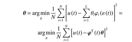
Considering the original nonlinear closed-loop system structure with one nonlinear plantf(·) and nonlinear feedforward controllerK(·), by replacing the nonlinear feedforward controller within a system with an equivalent linear time-invariant controller, which is in some sense the best possible linear approximation of the given nonlinear controller.This optimal linear approximation for a nonlinear feed-forward controller varies as a function of the input, being shown in Fig.2.

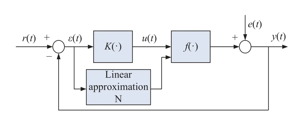
Fig.2 Approximated controller analysis

In Fig.2, an approximated linear controllerNis used to replace that unknown nonlinear feed-forward controllerK(·).

For analysis purposes, assume that the output of the nonlinear feed-forward controllerK(·) is a continuous function, denoted by

The goal is to optimality approximate the original nonlinear feed forward controller for a given input ε(t) by the output of a linear controller.This class of linear controller, denoted byN, is treated as a convolution form with integral operators.Thus the output of the linear controllerNis given by

The convolution kerneln(t)is chosen to minimize the mean squared error, defined by

Based on the above mean squared error (6), that optimal linear approximated controllerNsatisfies the following condition, reformulated in Theorem 1.

Theorem 1 There exists an optimal linear controller approximant solving the mean squared error in (6), with convolution kerneln∗(t).Then convolution kerneln∗(t)satisfies that

where ϕεN(τ) is the cross correlation between ε(t) and the approximated linear output, and ϕεK(τ) is the cross correlation between ε(t) and the original nonlinear outputK(ε(t)).

Proof Letn∗(t) be the convolution kernel of the optimal linear controller since the criterion in (6) is quadratic in the convolution kerneln(·).

For anyn, one has

Thus the detailed expression for errore(n)-e(n∗) is that

Asn∗(t) is the optimal approximant, one has

whereDε(t)=Nε(t)-N∗ε(t) is the linear difference operator betweenNandN∗.

Since the right-hand side of (9) is nonnegative for allDε(t), one has

As the convolution expression forNε(t) may be written as

Substituting (11) into (10), then

It is convenient to define:

Then (12) is simplified as that

Using the fact that the linear controllersNandN∗are all casual and stable, then one has

i.e.,

Since the above equation holds for arbitraryn-n∗, it holds that

Expanding (17) to get

i.e.,

3.3 Practical data-driven controller

Observing model inverse method in that optimization problem in (3),are collected through some physical devices, then one controller is constructed to achieve the data fitting, whatever its nonlinear or linear form.It means one expression aboutf(·) is approximately chosen to guarantee the cost functionJ(u(t)) is zero, so the model inverse method corresponds to one data fitting process, i.e., finding one form off(·) from the observed data.

Similarly, the approximated analysis method tells us that a nonlinear feed-forward controller can be approximated with one linear approximated form, which satisfies the requirement of Theorem 1.Based on (7), that linear approximated controller is an optimal form under the case of two equivalent cross-correlation functions.From this requirement, the linear controller can be chosen by the designers from different linear forms, for example,the commonly used linear proportion-integration-differentiation (PID) form, linear affine form, i.e.,

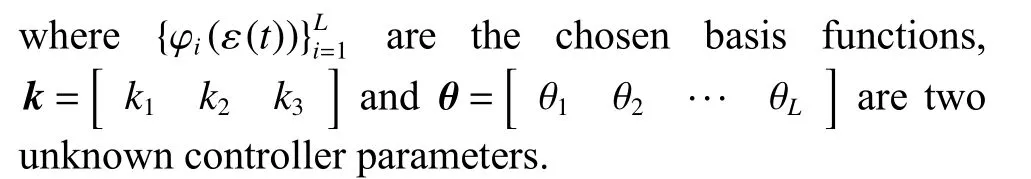
The problem of identifying those unknown controller parameters is solved while satisfying that requirement in Theorem 1.But in practice, the simple way of identifying the controller parameter vector θ depends on the leastsquares algorithm, i.e., solving the following optimization problem:

Due to space limitations, the detailed identification process is omitted.Here only the final result is given for that controller parameter vector:

Substituting this above controller parameter vector into that linear affine form and testifying whether that (7) is satisfied.

Observing (3) and above least squares criterion again,the only needed information are

and no prior message about that nonlinear plant is needed, so the goal is to extract one explicit form for that nonlinear controller with some chosen linear form, satisfying the requirement in Theorem 1.From the above description, all interesting topics are to get some messages about that nonlinear controller from the observed data, it corresponds to the idea of direct data-driven control.

3.4 Some considerations

Theorem 1 gives one linear approximated controller to replace the original nonlinear feed-forward controller only through its two sides, i.e., input-output signal.In our opinion, a special inputr(t) is chosen to excite that closed-loop system, and then one linear approximated controller is designed to satisfy that equity (7).

On the virtue of this optimal approximation to a nonlinear feed-forward controller, similarly, one linear plantMis also constructed to approximate the original nonlinear plantf(·).These two linear approximations can be implemented by two strategies, i.e., centralized strategy and distributed strategy, being shown in Fig.3 and Fig.4.

Fig.3 Centralized linear approximation

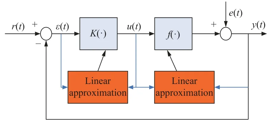
Fig.4 Distributed linear approximation

In Fig.3, i.e., centralized linear approximation, only one modular mechanism collects two kinds of data{ε(t),y(t)}to design a linear controller and linear plant simultaneously.But on the contrary in Fig.4, i.e., distributed linear approximation, two modular mechanisms are constructed within the above process.

Generally, through comparing Fig.3 and Fig.4 for centralized control and distributed control respectively,their main difference is the number of the designed controller.More specifically, for centralized control, one mechanism is used to control all the considered plants.But for distributed control, one plant is controlled by only the controller, so the number of the considered plants is the same as the number of the controllers.

4.UAV formation flight system

UAV formation flight has emerged as a prominent and evolving research area in recent years, encompassing a range of intriguing facets [24,25].These research topics contain high-level decision-making and low-level flight control.More precisely, UAV formation entails the coordinated deployment of multiple UAVs that share identical or similar specifications, following predefined rules to achieve effective task execution.UAV formation flight modes encompass autonomous reconfiguration, trajectory maintenance, and trajectory control.As illustrated in Fig.5, which depicts the structure of UAV formation flight.

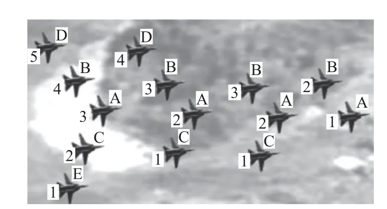
Fig.5 UAV formation flight structure

Fig.5 illustrates the necessity for the UAV group in cooperative formations to maintain stability and structural integrity over time.This requirement is met through the judicious selection of a formation control strategy.Currently, three primary approaches are commonly employed:

(i) Formation control based on behavior;

(ii) Formation control based on leader-follower;

(iii) Formation control based on virtual structure.

For the sake of simplicity, a detailed explanation of the second approach will be provided, as the principles of the other two approaches are similar to it.

The leader-follower flight mode, as depicted in Fig.6,involves the following process: initially, based on a predefined desired formation, the UAV group must maintain this formation structure in real time.Subsequently, the follower UAVs continuously receive and incorporate information regarding the leader’s speed, altitude, and heading angle.Using this information, the follower UAVs make adjustments to their positions to ensure they remain in alignment with the leader, thereby preserving the desired formation.

Fig.6 Leader-follower mode

The control strategy of UAV formation flight can be summarized as follows:

Step 1 The leader transmits necessary flight commands to the followers via data communication, including heading angle, speed, and corresponding formation information.

Step 2 The followers, taking into account their previous actions, compute the formation error signal, which is crucial for maintaining the desired formation.

Step 3 The followers utilize the information received from the leader to calculate the current separation distances between adjacent UAVs.

Step 4 By calculating deviations in velocity and heading angle between the leader and the followers, control rules are generated.These rules are then used to issue flight commands to the followers, enabling them to navigate along the prescribed trajectory.

These four steps constitute the fundamental structure of the formation flight control system as depicted in Fig.7.

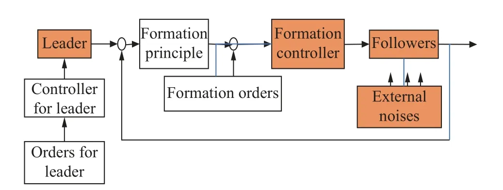
Fig.7 Formation flight control structure

5.Numerical example

In this numerical example section, some parts are extracted from Fig.7, i.e., follower, formation control,external noise, and the external input leader in Fig.8.Fig.8 is also regarded as a unit feedback closed-loop system, being similar to the one in Fig.1.

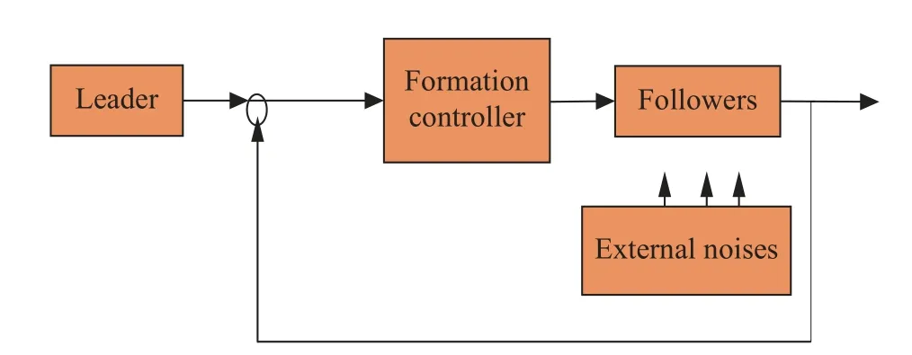
Fig.8 Extracted formation flight control system

In Fig.1 and Fig.8, the follower is the nonlinear plantf(·), the formation controller is the nonlinear controllerK(·) , input from the leader corresponds tor(t), and the external noise ise(t).

During the formation simulation, three UAVs exist,i.e., one leader and two followers, and the simulation time interval is 160 s.The original position, horizontal velocity, and heading angle are denoted as (xi,yi),vi, and φirespectively.The whole flight is divided into two stages.The first stage is in [0,80] s, and the second stage is in[80,140]s.More specifically, within the first stage, the leader flies in a straight and level flight with a constant velocity, and its heading angle is 0°.Similarly, in the sec ond stage, the leader will rotate around -10° at a constant angular velocity, but its flight velocity remains the same.

To avoid the identification process for that follower,two sides of data are collected around the formation controller, after one order from the leader is sent or excites the nonlinear closed-loop system.This order from the leader is chosen as a constant or one special signal, i.e.,square wave, shown in Fig.9.The corresponding output signal is measured and plotted in Fig.10.

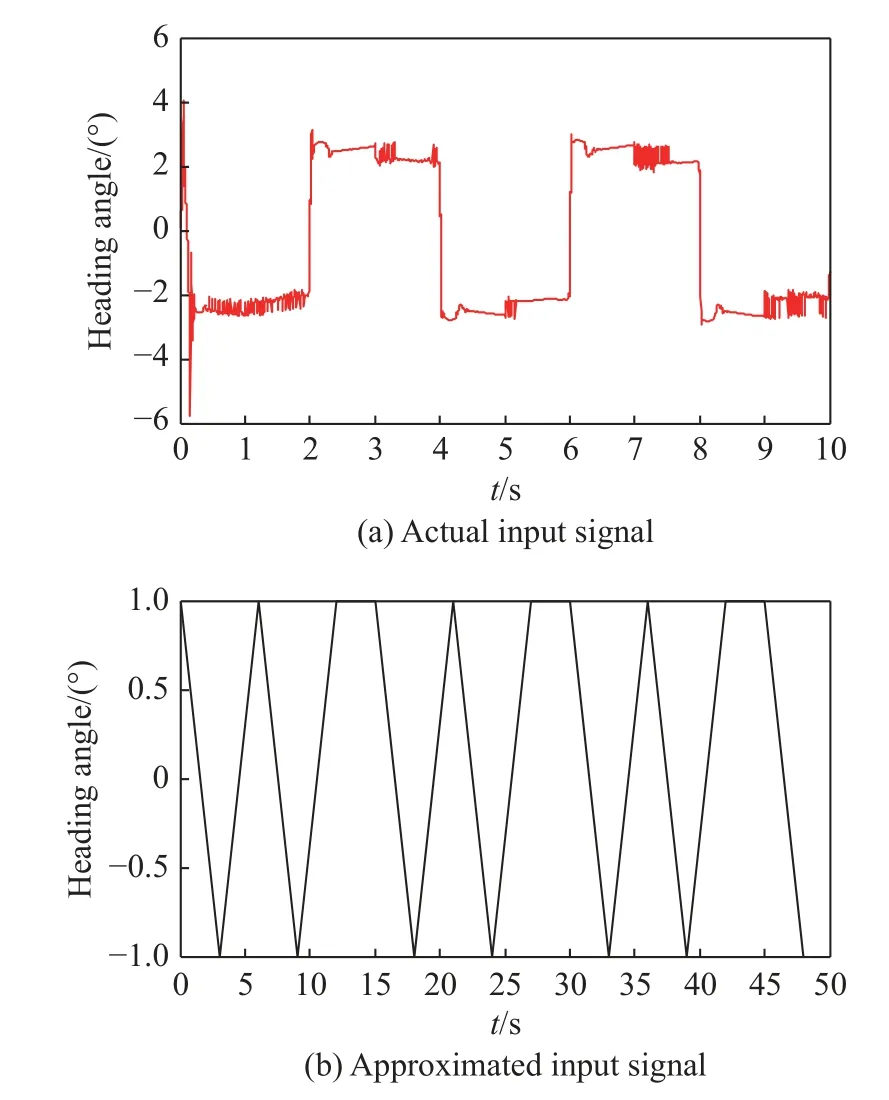
Fig.9 Applied input signal

Fig.10 Observed output signal

Based on the input signal and output signal in Fig.9 and Fig.10, the mission is to design one nonlinear form for that formation controller.Through using the proposed nonlinear direct data-driven control strategy, one approximated linear controller is applied to replace that nonlinear formation controller.Specifically, the commonly used linear PID form is used here, i.e.,

Then the mission is to change to design these three above unknown parametersk1,k2,k3from the input-output measured data.It corresponds to one data fitting problem, i.e., designing three parameters to guarantee the real output be same as the output in Fig.10.

In practice, the leader sends one order to those two followers, i.e., telling two followers to fly around the leader.The flight trajectory of the leader is the desired or expected flight path.After two followers receive the order from the leader, then two followers will modify their flight situations, and track the leader as soon as possible.According to the leader’s flight trajectory, the formation controllers will design the above three proportional-integral-derivative (PID) parameters, so that the two followers will fly near to the leader.Fig.11 shows the whole flight trajectories for the leader and two followers, and the horizontal velocity varying curve and heading angle varying curve are all plotted in Fig.12 and Fig.13.From Fig.11 to Fig.13, we see after two followers receive the order from the leader, they will fly near to the leader, then achieving the tracking goal perfectly.This tracking performance can be proven during the late 40 s when three flight trajectories are close to each other.Furthermore, to make the simulation more efficient,Fig.14 shows two flight trajectories.One is the flight trajectory for the leader, and the other corresponds to one follower’s trajectory.To connect it with the corresponding theoretical analysis, the leader’s trajectory is called the desired trajectory, and the follower’s trajectory is the real trajectory.These two trajectories approach closely after some seconds, during which the leader and follower communicate in a data link.

Fig.11 Whole flight trajectories for the UAV group

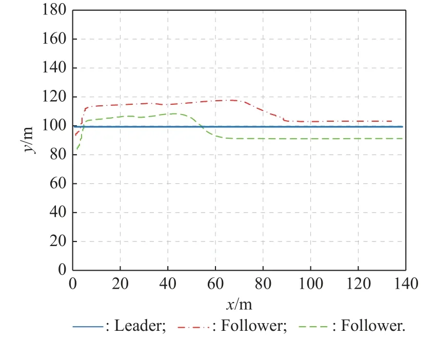
Fig.12 Horizontal velocity varying curve

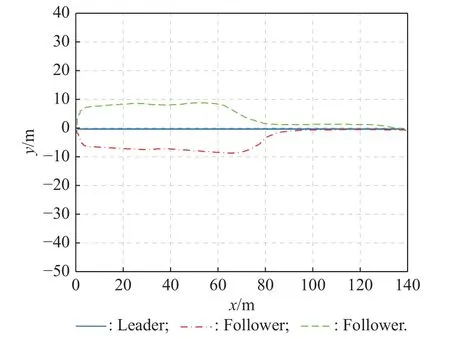
Fig.13 Heading angle varying curve

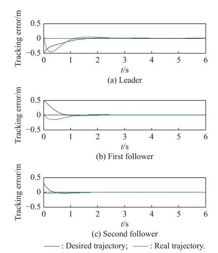
Fig.14 Two flight trajectories for leader and follower

6.Conclusions

Based on our previous contributions to direct data-driven control, this paper is concerned with nonlinear direct datadriven control for UAV formation flight systems.More specifically, to avoid any information about nonlinear plants, a nonlinear direct data-driven control is proposed to be two different forms, such as the model inverse method and approximated analysis method.The detailed derivations about the proposed control strategy are given from the point of theoretic aspect, and its application in UAV formation flight system is also given.Generally,stability analysis and computational complexity for nonlinear direct data-driven control strategy are our next work.