YOLOv5-Based Seabed Sediment Recognition Method for Side-Scan Sonar Imagery

WANG Ziwei, HU Yi, DING Jianxiang, and SHI Peng, *

YOLOv5-Based Seabed Sediment Recognition Method for Side-Scan Sonar Imagery

WANG Ziwei1), HU Yi2), DING Jianxiang3), and SHI Peng1), *

1),,100083,2),,,361000,3),,200444,

Seabed sediment recognition is vital for the exploitation of marine resources. Side-scan sonar (SSS) is an excellent tool foracquiring the imagery of seafloor topography. Combined with ocean surface sampling, it provides detailed and accurate images of marine substrate features. Most of the processing of SSS imagery works around limited sampling stations and requires manual interpretation to complete the classification of seabed sediment imagery. In complex sea areas, with manual interpretation, small targets are often lostdue to a large amount of information. To date, studies related to the automatic recognition of seabed sediments are still few. This paperproposes a seabed sediment recognition method based on You Only Look Once version 5 and SSS imagery to perform real-time sediment classification and localization for accuracy, particularly on small targets and faster speeds. We used methods such as changing the dataset size, epoch, and optimizer and adding multiscale training to overcome the challenges of having a small sample and a low accuracy. With these methods, we improved the results on mean average precision by 8.98% and F1 score by 11.12% compared with theoriginal method. In addition, the detection speed was approximately 100 frames per second, which is faster than that of previous methods. This speed enabled us to achieve real-time seabed sediment recognition from SSS imagery.

seabed sediment; real-time target recognition; YOLOv5 model; side-scan sonar imagery; transfer learning

1 Introduction

The identification of diverse seabed sediment categories is essential for marine resource exploitation and environmental information assurance of offshore operations (Zhu., 2021). Currently, the most common method of sea- bed sediment identification is based on surface sampling analysis and the depiction of sediment types. Marine remote methods based on acoustic technology, such as multibeam sonar, side-scan sonar (SSS), and subbottom profile, are used for areas with sediment type variability. The SSS system has been widely used because of its capability to produce an ‘acoustic image’ of the seabed, portability, and low cost (Dura., 2005; Coiras., 2007; Wang., 2018; Yan., 2021). The SSS system emits an acoustic wave and receives it after backscattering from the seafloor. Then, it constructs an image of the seafloor topography. The re- turned signal carries information related to the seafloor to- pography, including the sediment type (Collier and Humber, 2007). Under normal conditions, the returned sound wave becomes stronger at protruding, hard, and rough seafloors and weakens at recessed, soft, and smooth ones. In many investigations, SSS was used to identify the targetand classify sediments, especially in areas with variable se-diments. The full coverage swath of the SSS can effective- ly supplement sediment identification based on sampling. The SSS system has been successfully applied to seafloor microgeomorphology surveys (Chik, 2008; Greene., 2018), underwater ecological surveys (Gruzinov, 2019), underwater mineral resource exploration (Blondel, 2000), shallow-sea CO2bubble detection (Uchimoto., 2020), and habitat suitability analysis of mussel species (Flores., 2021).

In previous studies, the target recognition of SSS imagery mainly relied on human experience, which is very time- consuming. In addition, some critical information may be neglected in the complex sediment environment. Therefore, some scholars have studied the automatic identification of seabed sediment based on SSS imagery. Lamarche (2011) applied fuzzy c-means (FCM) classification algorithms to identify seascape classes and generate substrate classifica-tion maps for Tasmania, Australia. The use of FCM allow- ed the derivation of affiliation values for each unit in each class and helped define classes from complex and overlapping areas of the seabed. Xi. (2017) proposed an improved BP neural network to classify the SSS imageries of seabed sediment. They utilized the gray covariance matrix method to extract four kinds of seabed sediment texture characteristics and input them into a BP neural net- work optimized by an improved particle swarm optimization algorithm. Sun. (2020) proposed a probabilistic neural network (PNN) based on seabed sediment recognition from SSS imagery. The features of the gray co-occurrence matrix were selected as texture features. Color moments were used to represent color features combined as theinput matrix of PNN for classification. Compared with the traditional clustering method, the PNN algorithm increased the classification accuracy to 92.2%.

These methods are combined with the manual extraction of image features and machine learning classification me- thods. The data are then applied to SSS imagery recognition. However, this process is a time-consuming trial. In addition, some features might be missed in the search for the right target in most cases. Thus, the current approaches cannot completely represent the SSS imagery, which results in the poor robustness and weak generalization capability of the extracted features. With the rise of convolutional neural networks (CNNs), which can be used to analyze images after artificial segmentation without feature extraction, some researchers have applied CNNs for seabed identification. Berthold. (2018) proposed the application of CNNs to the automatic classification of sea-bed sediments based on SSS imagery. The CNN model has a simple structure that mainly consists of two convolutionaland two pooling layers. Experiments were conducted usingpatch-wise classification with ensemble voting. An accuracy of 83% for coarse sand sediment prediction but a poor accuracy (11%) for fine sediment was achieved. Qin.(2021) used a CNN with different depths to classify sediments in a small seabed acoustic image dataset and used the gray Cifar-10 dataset for pretraining. In their experiments,the best result obtained by fine-tuning ResNet was 3.459%.Luo. (2019) constructed two CNN classifiers to classify small-scale seabed acoustic image datasets. One is the shallow CNN classifier based on LeNet-5, and the other is the deep CNN classifier based on AlexNet. The shallow CNN features accuracy better than 87.5%, and that of deep CNN is 66.75%.

However, all the above works obtained images with a single sediment type as the input, which needed image pre- processing. Moreover, given the live time needed to identify seabed sediments in the SSS imagery for real-time work, the detection efficiency has higher requirements. To solve this problem, we introduce You Only Look Once version 5 (YOLOv5) (Ultralytics, 2020) for marine sediment identification. This report shows for the first time the application of YOLOv5 to the research of target detection in seabed sediment SSS imagery.

YOLO is a target detection algorithm first proposed by Joseph Redmon and others in 2016. The YOLO series of target detection algorithms have been optimized to become faster and better and updated to the fifth generation as of 2021. It has also been applied in many fields, such as me- dical imaging, road traffic signs, and face mask detection. Ozturk. (2020) proposed a YOLO-based model to de- tect and classify novel coronavirus 2019 (COVID-19) casesin X-ray images. The model used original chest X-ray images for automated COVID-19 detection. The goal was to provide an accurate diagnosis for binary classification (COVID for no findings) and multiclassification (COVID for no findings on pneumonia). The accuracies of classification were 98.08% and 87.02%. Dewi. (2020) used six YOLO-based networks for traffic prohibitory sign re- cognition. The experimental results showed that YOLOv3- SPP outperformed the other models in terms of the mean average precision, but it needed more time. Kumar. (2021) applied the improved YOLO algorithm to face mask recognition. To propose a new face mask detection algorithm with high accuracy in a limited computing resource environment, they selected four minor variants of the YOLO algorithm. They proposed a new architecture modification in its feature extraction network, which improved the over- all performance, especially increasing the mAPs of tiny- YOLOv3 and tiny-YOLOv4 by 4.12% and 2.54%, respectively. Sun. (2021) adopted YOLOv3 for seabed sediment identification and added transfer learning. The average precision (AP) can reach 84.39% in less than 0.2s. However, certain shortcomings were still noted. They fixed the original SSS imagery to 416pixel×416pixel, which cannot be used to recognize large-sized and multipletargets. Meanwhile, the seabed sediment classification was incomprehensible, the discussion of experimental results was insufficient, and the inference speed needed to be im- proved. Yu. (2021) applied YOLOv5-S to wreck and container identification. They added a transformer moduleand downsampling to improve the accuracy and efficiencyand finally attained a mAP of 85.6%. However, the lack oforiginal samples allows detectors to learn more easily features that are not excellent enough, which leads to overfitting and limits the recognition accuracy.

Our research work aimed to overcome all the above chal- lenges. The main contributions of this paper are as follows:

1) The proposed model is fully automated and has an end-to-end structure. The entire imagery was inputted into the network without a separate step of manual feature extraction.

2) The feasibility of real-time recognition of sonar imagery by YOLOv5, which can produce real-time recognition results during ocean surveys, was proven.

3) Different methods in the YOLOv5 target detection structure were compared by a large number of experiments. The performances of five different methods were shown and analyzed directly. The findings will serve as guiding principles for readers in selecting the appropriate method in practice.

2 Methods

The main steps of our method include data collection, training and recognition. First, we processed the original SSS data file (such as XTF, SDF, JSF, HSX, MSTL, or QMips) with parsing software to reconstruct the SSS video. One frame was removed from every 100 frames to obtain the original dataset. Then, various methods were added, and different variants of the YOLO model were trained using image to acquire the best weight parameters. Finally, the seabed sediment was identified on the test set and analyz- ed based on the evaluation index. Fig.1 provides a detailed flowchart of the training and detection process used in this paper.

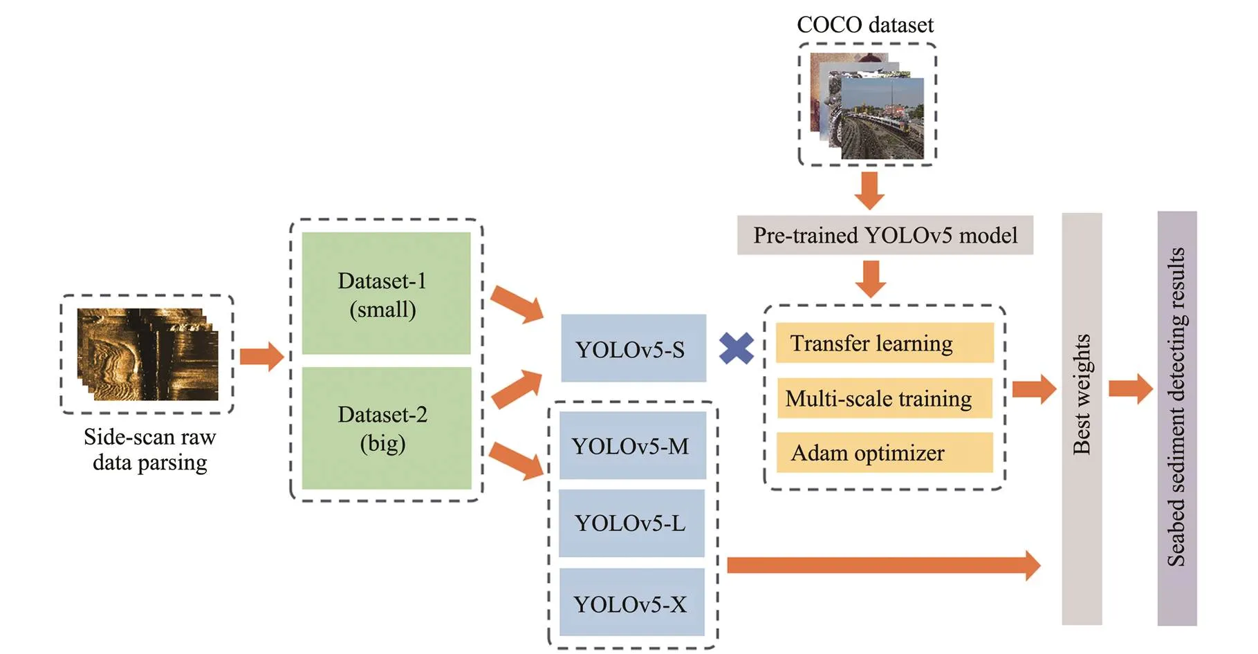
Fig.1 Flow chart of the methods used in this study.

Table 1 shows the environment where the models were trained and tested in this paper. To reduce the hardware de-vice requirements, we set the epoch to 4, the initial learningrate to 0.01, the momentum value to 0.937, and the weight decay to 0.0005. The training period settings were varied in accordance with different experimental designs. During the training process, we adjusted the SSS images to 1280 pixel×1280pixel.

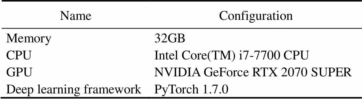
Table 1 The experimental results using different methods

2.1 YOLO Series Models

YOLO is a deep neural network model for object detec-tion. The object detection task consists of two parts: objectclassification and object location in the image. Unlike pre-vious target detection algorithms, such as region-based CNN (R-CNN), YOLO uses an end-to-end design approach that transforms object detection into a regression problem. It obtains the entire input image through one neural network and directly obtains the bounding box coordinate informa-tion and probability of the category to which each bounding box belongs. As only one network is used in the whole detection process, it can be directly optimized end-to-end (end-to-end: the original data are inputted; the final result is outputted, applied in feature learning, and integrated intothe algorithm without any separate processing). YOLO offers a new solution to the object detection task: combining location and classification tasks, scanning an image once, using a deep neural network to extract features and classify location, enabling real-time detection, and maintaining a high mAP.

The YOLO network consists of three main components (Bochkovskiy., 2020):

The backbone is a CNN that aggregates different fine- grained images and forms image features.

The neck is a series of network layers that combine and transfer image features to the prediction layer.

The head predicts image features, generates bounding boxes, and forecasts categories.

The loss function of YOLO comprises three parts: box, objectness, and classification losses. Box loss contains twoparts: the coordinate center error and the error of width and height. When a box predictor is responsible for a ground truth box, the box coordinate error will be penalized. The larger the Intersect over Union (IOU) values, the closer the box is to the true position. Objectness loss is calculated as the confidence error. Confidence is used for the bounding box, and given that each grid cell has multiple bounding boxes, individual grid cells will have a corresponding num- ber of confidences. Classification loss is calculated from the probability of the predicted category and true proba- bility. When an anchor box of a grid cell is responsible for a real target, only the bounding box generated by this anchor box will be used to calculate the classification loss function.

YOLOv1 is fast and simple, but it also has disadvantages:1) difficult detection of overlapping targets; 2) incapability to accomplish multiple tag detection of a target; 3) poor effect on small objects in the image. Based on YOLOv1, a series of improved versions was proposed. YOLOv5 is the latest version, and it increases the speed while ensuring im- proved accuracy and offers four models with increasing complexity.

Compared with previous works on SSS-based seafloor sediment identification, YOLO is distinctly significant be- cause it considers an entire image as input and can recognize it in real-time. It no longer requires feature downsca- ling using a suitable feature selection method. In addition, the CNN included in YOLO can extract more features to compensate for certain characteristics missing from the fea- ture set extracted by manual selection in a complex substrate environment, which is beneficial for marine substrate re- cognition.

2.2 Multiscale Training

Normally, the size of input data is fixed and remains un- changed during training. However, the scale and range of seabed sediment recognition targets differ and have indeterminate boundaries (Lucieer and Lucieer, 2009). For ex- ample, the size of a rock can vary from several to hundreds of meters. If each image is resized to the same size during training, the detection effect will be poor. Therefore, this paper introduced a multiscale training method to improve the detection performance of the proposed model. In the basic network part, the feature image is often smaller than the original one, which makes the feature description of small objects difficult to capture by the detection network. We randomly changed the training data size to give the network some adaptability. By inputting larger and more images with different sizes for training, the robustness of the detection model to the size of an object can be improved to a certain extent. The multiscale training method provides a comprehensive model detection capability for small- and large-resolution sonar imagery.

2.3 Optimizer

Most deep learning algorithms involve some form of op- timization, which refers to the task of changingto mi- nimize or maximize the function(). The function to be minimized is usually called the loss function. The training model searches for a parameter combination that minimi- zes the loss function of the training set.

This paper used two optimization functions, namely, thestochastic gradient descent (SGD) with Nesterov momentum and Adam SGD with Nesterov momentum (Sutskever., 2013), which is a variation of the momentum algorithm. The difference between Nesterov and standard momentums is reflected in gradient calculations. In Nesterov momentum, the gradient is calculated after the application of current velocity. Thus, Nesterov momentum can be interpreted as the addition of a correction factor to the standard momentum method. Adam (Kingma and Ba, 2014) is an adaptive optimization algorithm for learning rate. Its advantages have two main aspects. First, compared with the standard SGD, Adam considers momentum to accele- rate the training process. Second, it adopts a bias correction as the constraint of the learning rate.

2.4 Transfer Leaning

The ideal scenario for machine learning is to have a weal- th of tagged training instances with the same distribution as the test data. In general, the more complex the network structure, the larger the number of training samples and the better the model performance. As the SSS dataset used in this paper lacked a sufficient number of seabed sediment samples, the model may exhibit poor overfitting and gene-ralization capability. Therefore, this paper trained and optimized a network model through transfer learning to improve the model training efficiency and validation perfor- mances.

Transfer learning applies the knowledge learned from a specific dataset (called source domain) to a target domain. Retraining a complex network model requires many data, computational, and time resources. Transfer learning can share the model parameters already learned to the new mo- del through transfer to accelerate and optimize the learning efficiency of the model, reduce repeated work and the dependence on target task training data, and improve the model performance (Zhuang., 2021).

In previous studies, transfer learning strategies based on SSS imagery have been applied to the classification and target recognition of underwater targets (Yulin., 2020; Qin., 2021) In our experiments, we used COCO (Mi- crosoft, 2017), which is widely adopted for image recognition transfer learning, as a preprocessed dataset. AlthoughCOCO is distinct from the seabed sediment imagery dataset, and unsuccessful knowledge transfer is possible, it is a meaningful attempt because of its large amount of high- quality labeled images. We trained the model on COCO and migrated it to our target task as a pretrained model.

2.5 Model Evaluation Metrics

To quantitatively evaluate the performance of the selec- ted models, we used some quantitative indicators, including precision, recall (R) rate, mAP, F1 score, and frames per second (FPS) (Padilla., 2020; Li., 2021).

2.5.1 Precision () andrate

True positive (TP) is the number of positive samples correctly identified as positive. False positive (FP) is the number of negative samples incorrectly identified as positive. True negative (TN) is the number of negative samples correctly identified as negative. False negative (FN) is the number of positive samples incorrectly identified as negative.is the percentage of correctly identified seabed sediment samples among the identified images being considered for a certain type of sediment. The calculation formula is as follows:

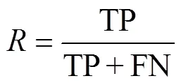
refers to the proportion of correctly identified positive samples in all positive samples. The calculation formula is as follows:

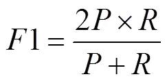
2.5.21 score

1 score is a measurement index of classification pro- blems. It considersrate and accuracy to be equally important.1 score is often used as the final evaluation me- thod in some machine learning contests with multiple classification problems.

2.5.3

Thecurve is the curve of horizontal and vertical axes withandas the coordinate system, respectively.is the area of the closed graph formed by the line parallel to thecurve’s horizontal and vertical axes. The better the effect of the target detection algorithm, the higher thevalue.

is theof all sediment categories in the dataset, and it takes values between 0 and 1. The better the performance of the algorithm, the larger the value of. Theis the ratio of the intersection and concatenation of the prediction frame and ground truth. By comparing thewith a given threshold, we can classify the detection as correct or incorrect. If≥, then the detection is considered to be correct. If<, then the detection is considered incorrect. In this paper, we set the thresholdas 0.5.

Thewas used to measure the accuracy of object detectors over all classes in our dataset. Theis theof all classes (Ren., 2017), that is,

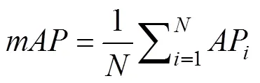
whereAPis thein theth class, andis the total num- ber of evaluated classes.

2.5.4 FPS

FPS is a definition in graphics that indicates the number of FPS transmitted. In video images, it refers to the number of FPS that the picture transmits. The higher the FPS, the smoother the displayed action will be. FPS is used in target detection algorithms to evaluate their detection speed. A large FPS indicates a fast detection speed. In general, when the FPS of the model exceeds 30 frames, real-time processing can be achieved (Ma., 2019; Li., 2021).

3 Experiments

3.1 Experimental Dataset

The experimental data in this paper were derived from the Klein 3000 SSS system, which adopts a dual-frequency sonar (100 and 500kHz) while maintaining a high target identification resolution at close ranges. The data were collected from the Taiwan Strait between 2012 and 2015. The water depth of the survey area was approximately 10 –35m. The side-scan raw data (the data format is XTF) were parsed with SonarPro software. In this paper, 207 imageries of marine substrates containing sand waves, rocks, and sandy silt with a size of 1280pixel×720pixel were selected. Here, we used two typical seabed categories as labels to prove our approaches. We used the popular image labeling software LabelImg to label side-scan images. The software saves the image resolution, pixel coordinates of the upper left and lower right corners of the border, and the category information of the substrate into a TXT file. A total of 216 reef labeling boxes and 125 sediment labeling boxes were used. Fig.2 shows several examples of manually labeled images.

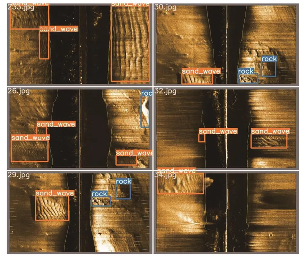
Fig.2 Several examples of the labeled dataset.

Given the small dataset, to avoid the high dependence of the model performance on the selected test dataset and to fully use all the data, we applied the-fold cross-validation (KFCV) method in the training and evaluation of each experiment. In the KFCV, the data were divided intopieces, and the training model combined-1 pieces of data as the training set and the remaining one piece of data as the test set. The above process was repeatedtimes. For each repetition, one data piece was used as the test set, and the average score of the model initerations was con- sidered the overall score. Our study applied avalue of 5, and the data were divided into five parts for cross-validation (Fig.3).

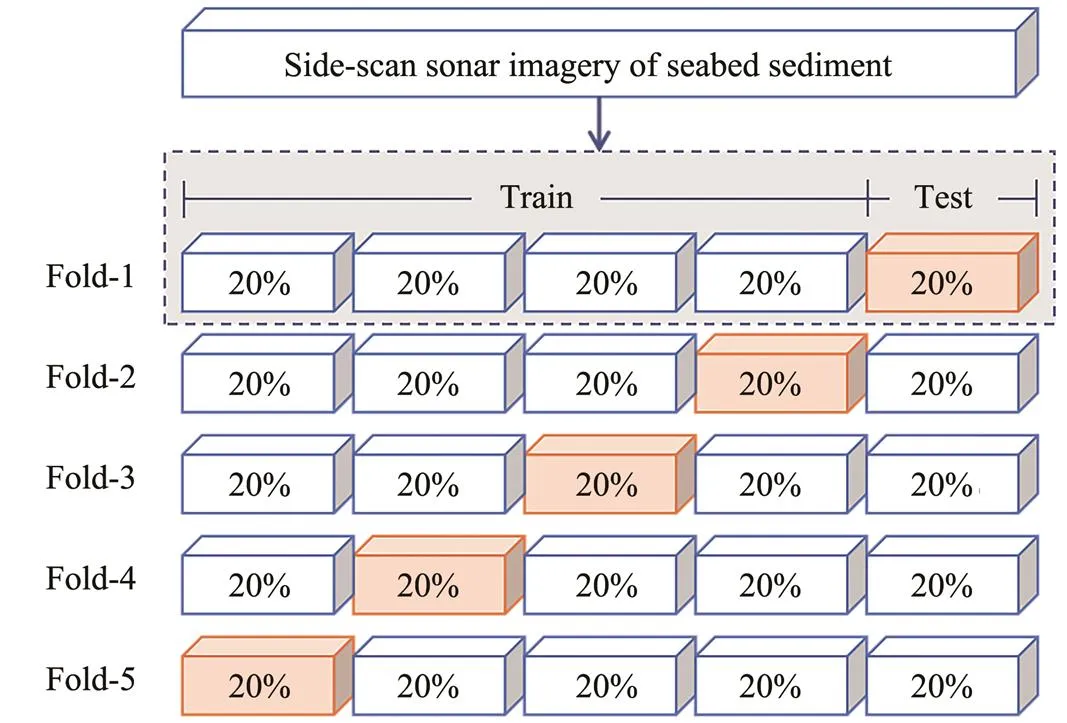
Fig.3 5-fold crossing-validation used in this study.

3.2 Training and Detection

In previous reports, no researchers used YOLO for SSS seabed sediment identification. Thus, we needed to prove its feasibility. First, we selected 50 images with relatively concentrated targets from the total dataset as Dataset-1 (Table 2). We applied the five-fold cross-validation method and randomly picked out 40 images from the selected images as the training and verification sets. The remaining ten images were used as the test set. The YOLOv5-S network model was trained for 2000 epochs. The bounding box, objectness, classification losses, andwere obtained in the training process. As shown in Fig.4(a), the three losses showed a downward trend overall. In the beginning stage of training, the loss value decreased signi- ficantly, which indicates that the learning rate was appropriate and the gradient descent process was carried out. The loss change stabilized until 1000 rounds and finally reached 0, verifying thatwas on the rise overall until it started to stabilize at the value of 1 in round 1000. The burr in the curve was due to the batch size. The larger the batch size setting, the smaller the burr is. The data of each batch were equivalent to different individuals (Fig.5) of batch data with a size of 4. Fig.4(b) shows thecurves under the current experimental conditions, and the abovewas derived from the area under thecurve.

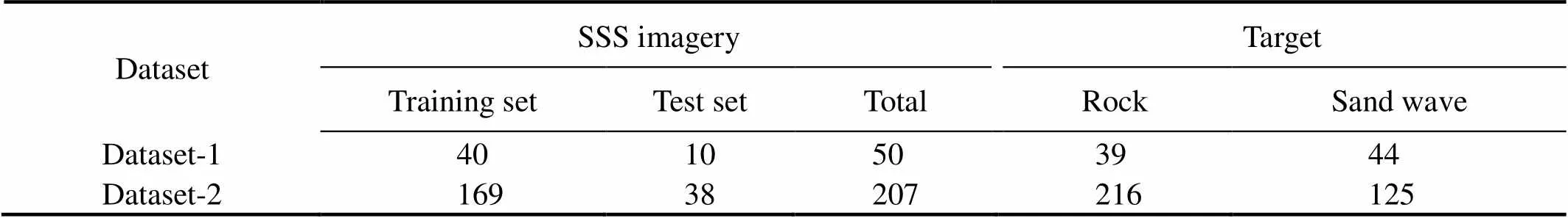
Table 2 Images and targets number of SSS datasets

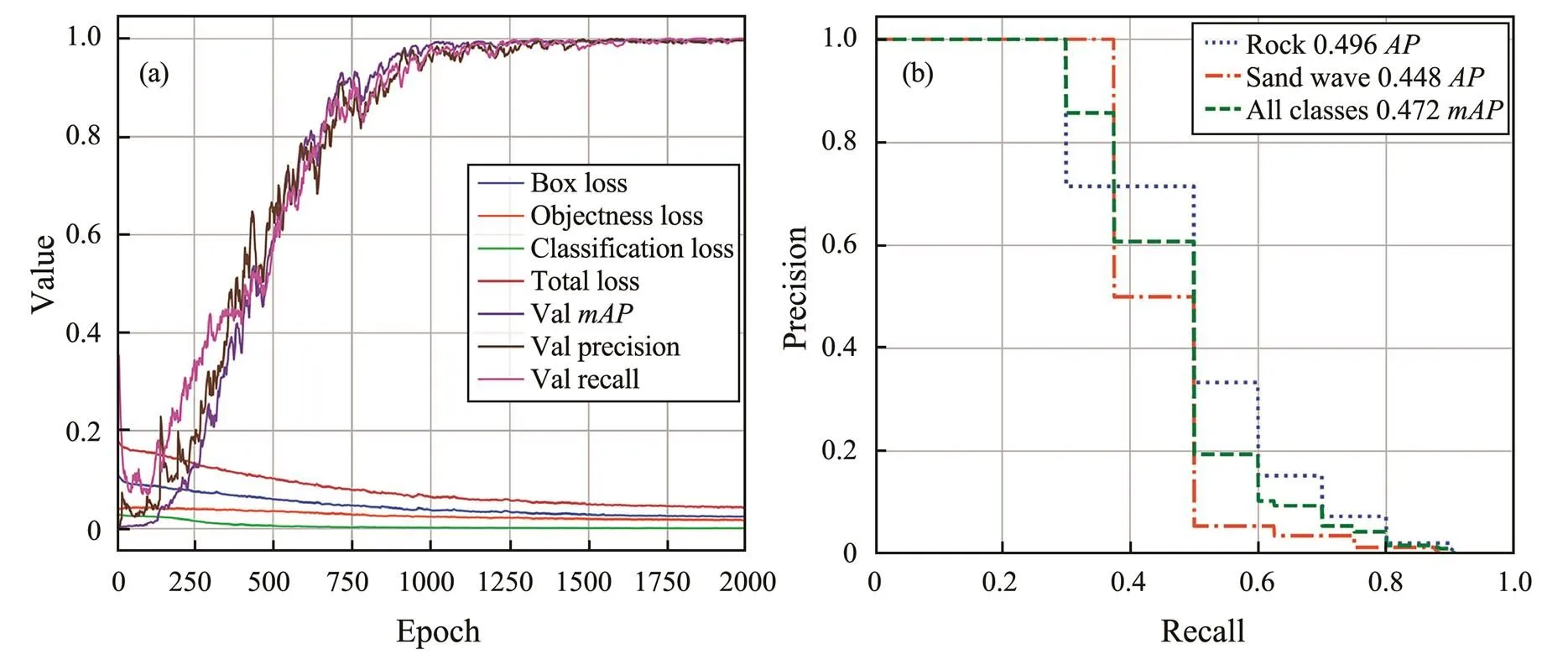
Fig.4 (a) Box loss, objectness loss, classification loss, total loss at training and precision, recall, mAP at validation using Da- taset-1 under epoch 2000. (b) The P-R curve of rock, sand wave, and all classes.

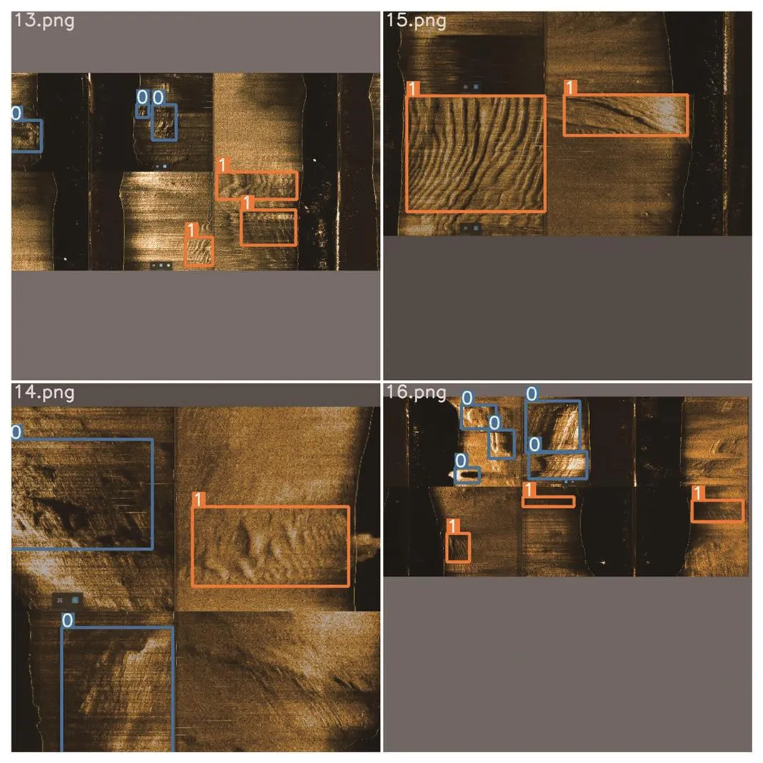
Fig.5 A batch data with size 4.

The weight parameters obtained at 500, 1000, 1500, and 2000 epochs were tested. The identification results are shown in Fig.6, where reefs and sand waves are delineated.The test evaluation indexes are shown in Table 3. Thewas 35.36% at 500 epochs. When the epoch was above 1000, the verifiedshowed a small difference of 0.7%. The decrease in the total loss value became stable after 1000 rounds of training. However, with the gradual increase in the1 score, the comprehensive evaluation index ofrate andand performance of weight parameters improved in this dataset. Therefore, the testtended to be stable during loss stabilization. In addition, increasing the epoch has limited improvement in the detection effect. Therefore, in subsequent experiments, we set the epoch number for training to 1000. When the epoch number was 2000, the verifiedcan reach 99.87%, and thein the test set was 51.26%, showing a difference of 48.61%. Thus, the modelhas a weak capability to recognize and generalize new seabed SSS imageries. The experiment in this section showed that the YOLOv5 target re-cognition algorithm can recognize seabed sediments based on SSS imagery, and its feasibility was proven.

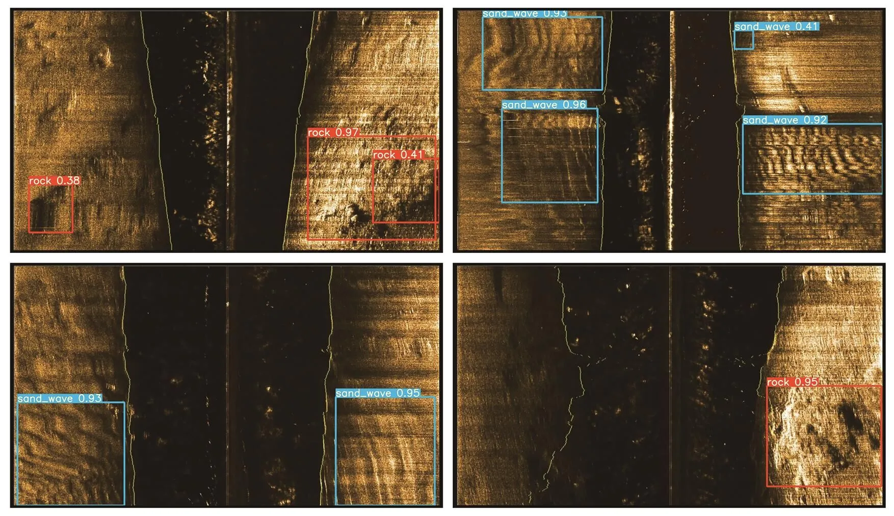
Fig.6 Identification results of the model weights obtained using Dataset-1 under epoch 1000.

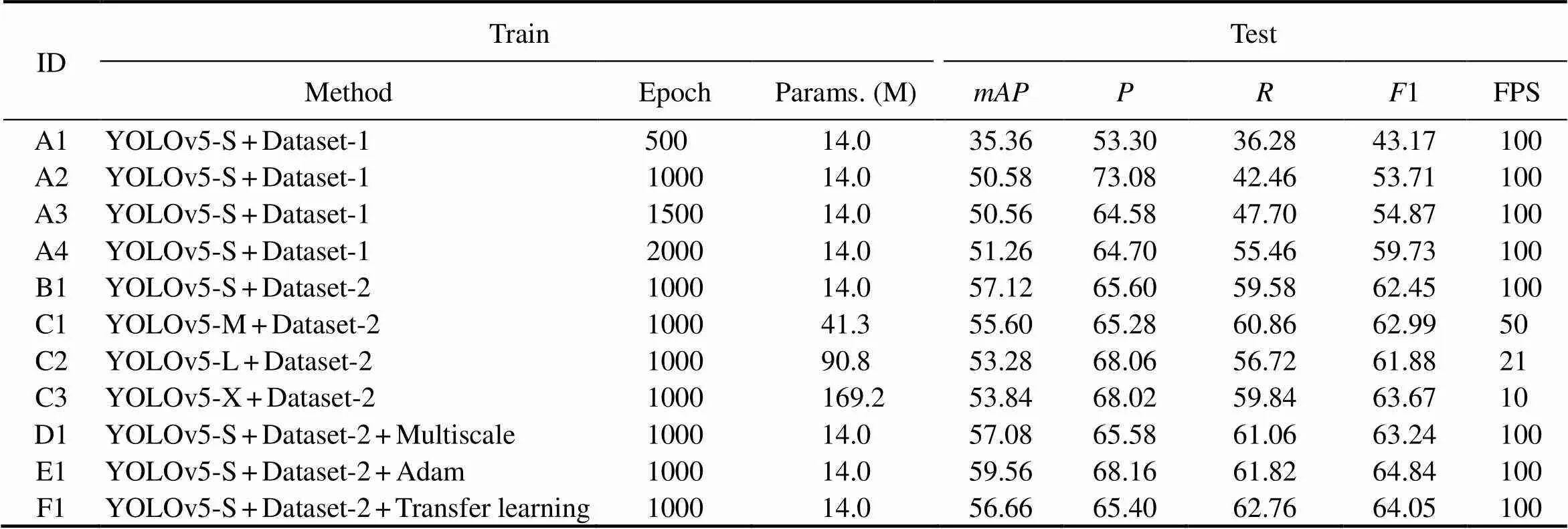
Table 3 Experimental environment

3.2.1 Influence of the number of images

Two experiments were designed in this section. The train- ing and test sets were expanded to four times the original size. The verification and training sets both had 169 pieces, and the test set had 40 pieces with 2000 rounds of training. The training process and test results were compared with those of the original experiment. As shown in Fig.7, in the training process, the loss decreased more rapidly after the expansion of the dataset. When the training reached 500 rounds, the loss decreased to a stable level, and theof the verification set also stabilized. However, the original dataset required 1000 rounds for the loss to decline and become stable. Then, we used the best weight parameters generated after 1000 epochs for testing. As shown in Fig.8, the metrics of seabed identification results significantly improved after the expansion of the dataset. Compared withthe original experimental test results under the same epoch number (1000), the test,1 score, andincreased by 6.54%, 8.73%, and 17.12%, respectively.decreased by 7.48%, which may be due to the small number of side- scan imagery for testing the small dataset. Sample selection also had a certain influence on the results.

3.2.2 Influence of different models

To investigate the influence of network models of different complexities on the recognition results, we set up four groups of experiments using YOLOv5-S, YOLOv5-M,YOLOv5-L, and YOLOv5-X for training. The hyperpara- meters of the four experimental training groups were the same, and the epoch number was 1000.

In this section, we used smoothed curves to show the trends more intuitively. First, as shown in Figs.9(a)–9(c), under each model, the overall loss showed a downward trend and converged to 0 when training up to 1000 rounds. Among the three losses, the objectness loss showed the largest difference between different models. The difference in loss value was relatively large. The more complex the model is, the lower the loss value and the faster the convergence. The other models exhibited a relatively slow loss decline. Then, as shown in Fig.9(f), theexhibited an upward trend. The trend flattened out after 500 iterations and reached 99.7% at the end. YOLOv5-S, YOLOv5-M, and YOLOv5-L network models performed better than YOLOv5-X in terms of,, and. We tested the best weight parameters trained by different models under 1000 epochs in the test set. As shown in Fig.10,was the highest in the YOLOv5-S model (57.12%). Between the three models, the higher-complexity model had a lowerthan the simplest model, with a difference of 3.84%. In addition, YOLOv5-S obtained the smallest weight parameter, and its FPS can reach 100. Therefore, we used the YOLOv5-S model in the subsequent experiments.

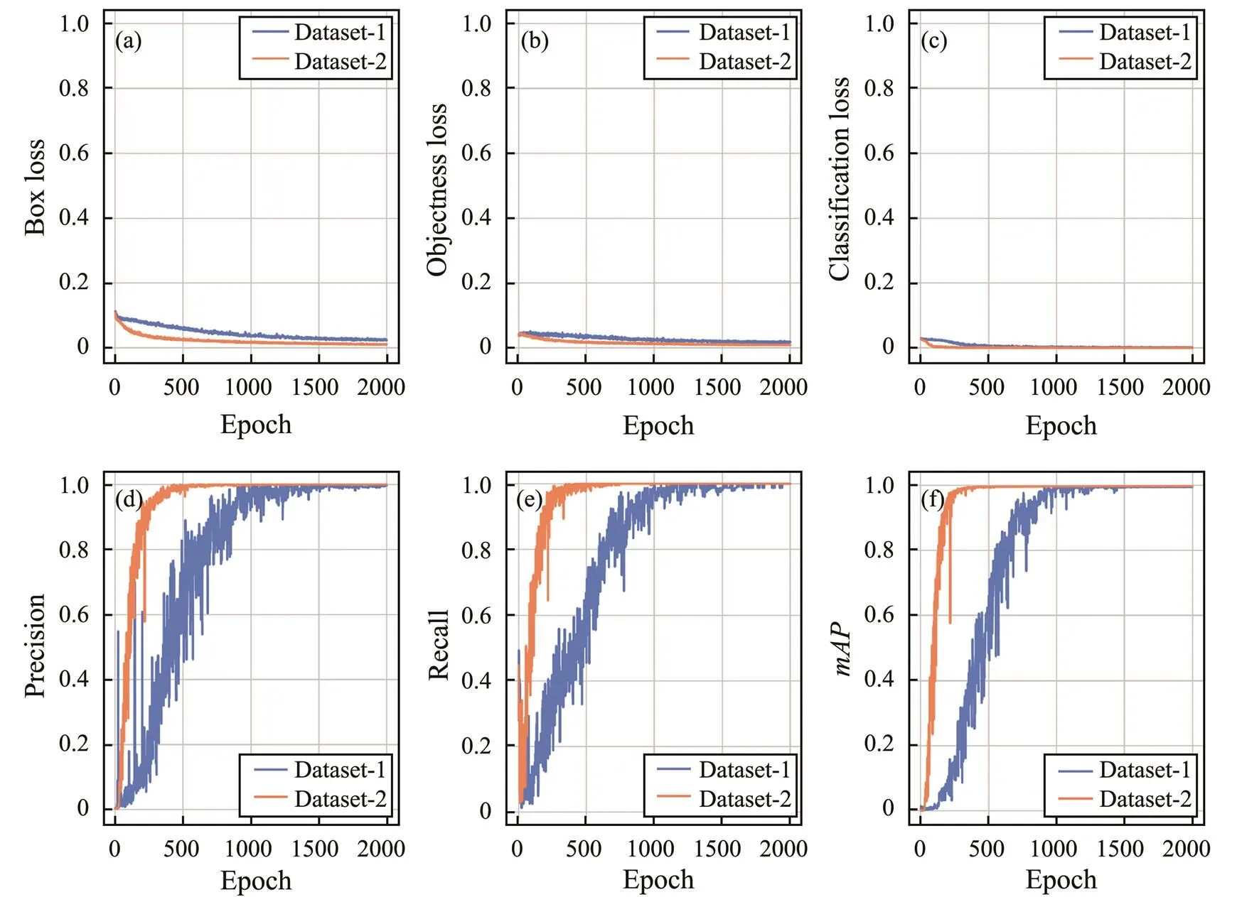
Fig.7 The variation of training and validation metrics for Dataset-1 and Dataset-2.

3.2.3 Influence of multiscale training

In this section, the experiment was compared with the original one by the addition of a multiscale training method.In the training process, the difference between the two me- thods was evident. After the addition of multiscale training,the loss decreased slowly. A great difference was observed between the objectness and box losses (Figs.11(a) and 11 (b)), but the difference in classification losses is not signi-ficant (Fig.11(c)). Figs.11(d)–11(f) verify that the convergence of,, andwas relatively slow and finally reached 98.91%. Then, the test was carried out, as shown in Fig.8. Theof the comparative experiment decreased by 0.04%. The addition of multiscale training did not improve the test, possibly because the target size in seabed sediment SSS identification was not fixed, and the boundary was unclear, unlike traffic sign detection using the YOLO algorithm. Meanwhile, the1 score showed a small improvement of 0.79%.

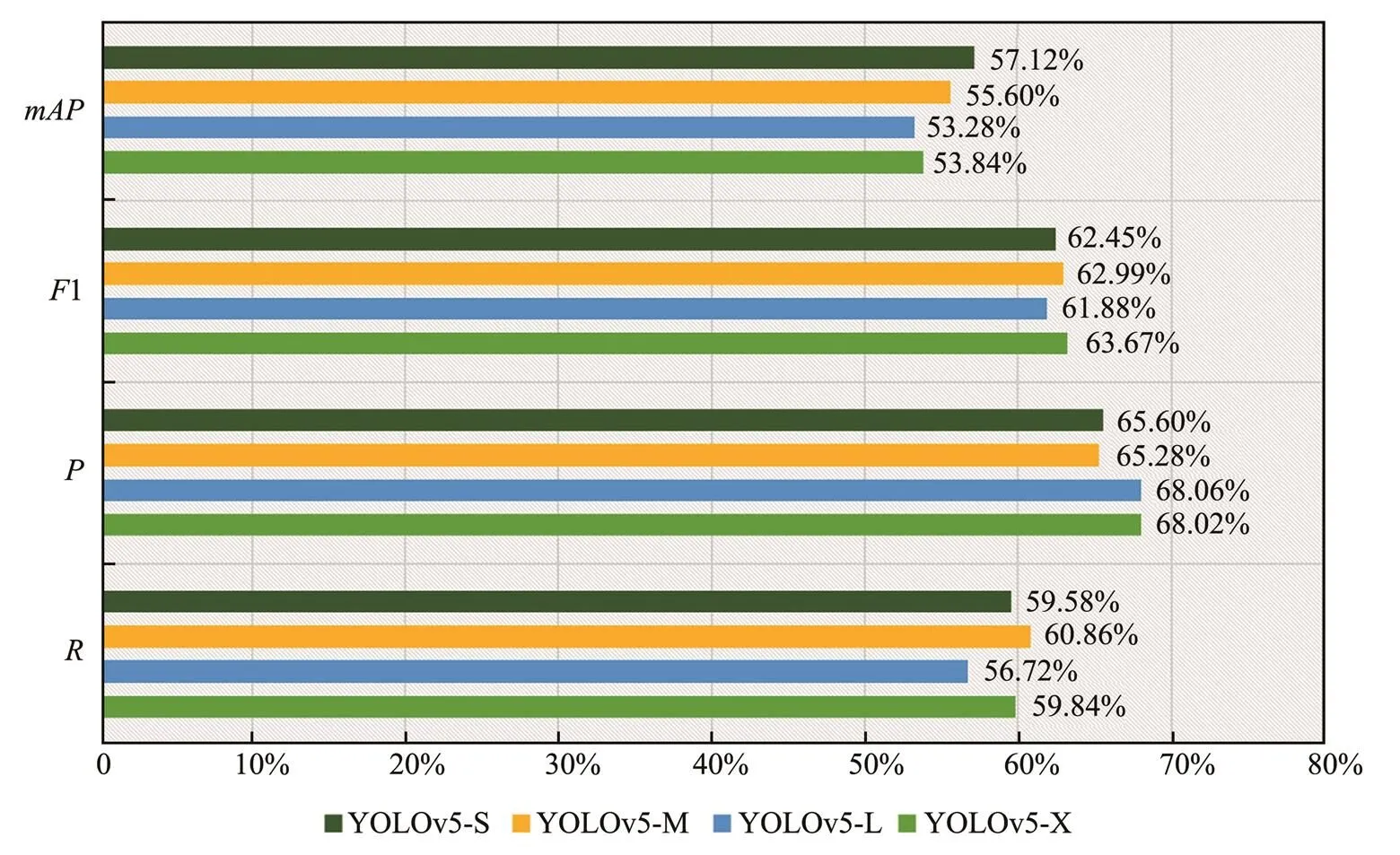
Fig.10 Comparison of the results of experiments A2, C1, C2, and C3.

3.2.4 Influence of the optimizer

YOLOv5 used an SGD optimizer by default, and Adam was also used for training in this experiment. Figs.12(a)–12(c) show that when SGD was used for training, the loss value decreased relatively quickly, and it decreased evidently under the epoch number of 300. With the Adam op- timizer, box and classification losses decreased re mark- ably in epoch 100. The best weight parameters obtained at 1000 epochs were used for testing. Fig.8 shows that when Adam was used, the,1 score,, andincreased by 2.44%, 2.39%, 2.56%, and 2.24%, respectively. Thus, the application of Adam optimized the test evaluation indexes. In this dataset, the overall performance of the results improved with the use of Adam.

3.2.5 Influence of transfer learning

In this experiment, transfer learning was performed using the models trained on the COCO dataset. Figs.13(a)–13(c) show three loss values. After the addition of transfer learning, the loss values were relatively low. Figs.13(d)–13(f) reveal that the convergence rate of the indicators was fast because of transfer learning. Fig.13(f) displays thattended to be stable at epoch 500 compared with that of the original experiment. Then, we used 500 and 1000 epochs to test the weight parameters and the results (Fig.8). With the same 1000 rounds, transfer learning did not improve theand decreased it by 0.46%. However,it improved the1 score by 1.6%. Consequently, the transfer learning of different datasets can also be successfully applied to seabed sediment identification and improve de- tection performance.

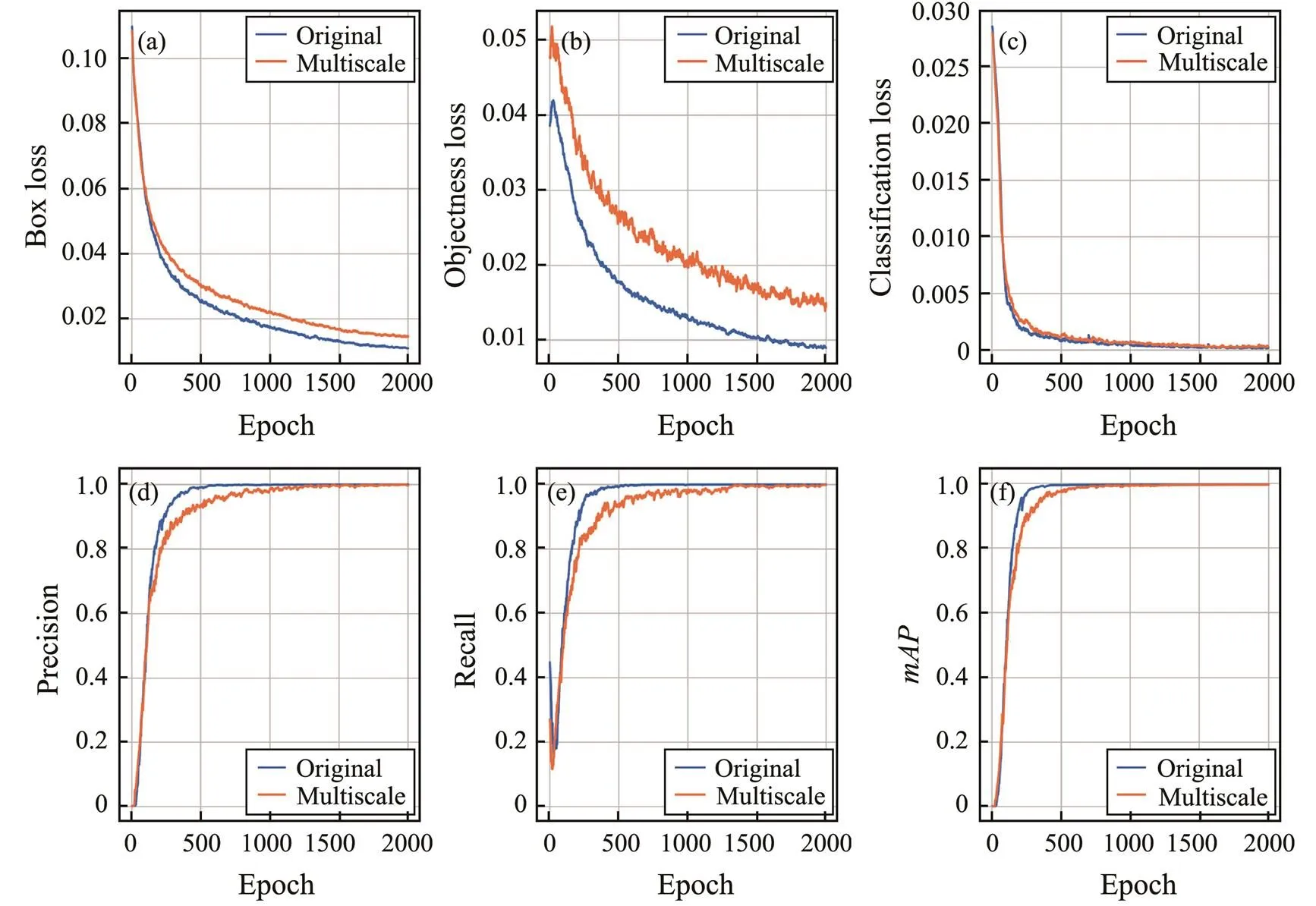
Fig.11 Variation of training and validation metrics of adding multiscale training.

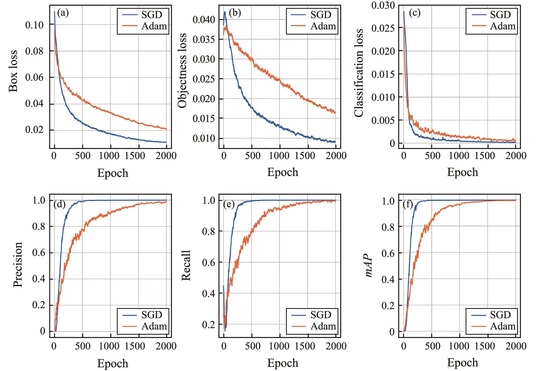
Fig.12 Variation of training and validation metrics of using Adam.

4 Discussion

Table 3 shows the influence of incorporating methods, such as expanding the dataset, multiscale training, changing the optimizer, and transfer learning, on the identification of seabed sediment based on SSS imagery. First, scaling the dataset to up to four times improved theby 6.54% and the1 score by 8.73%. Complex YOLOv5 net- work models can improve the recognition effect and affect the recognition speed, which is not conducive to rea- lizing real-time ocean bottom identification. YOLOv5-S had the smallest weight parameter size and highest recognition rates. It can detect a single image at a speed of 10 ms, which meets real-time requirements, and has relativelyhigh accuracy. YOLOv5-M reduced the FPS to 50 but also met the need for real-time target recognition. YOLOv5-L and YOLOv5-X models had many parameters that are unsuitable for embedded hardware devices, and their FPS is lower than 30, which does not meet the requirements of real-time identification. Second, multiscale training did not improve the performance ofin this dataset. Changing the optimizer to Adam improved the overall test me- trics. Finally, YOLOv5 can be applied to the identification of marine substrates based on SSS imagery. Meanwhile, the application of a large dataset, Adam optimizer, and the YOLOv5-S network model enabled the detection to meet the real-time requirements and improved the accuracy. They also improved the,1 score, andby 2.44%, 2.39%, and 2.56%, respectively. In addition,increased by 2.24%, and FPS reached 100.

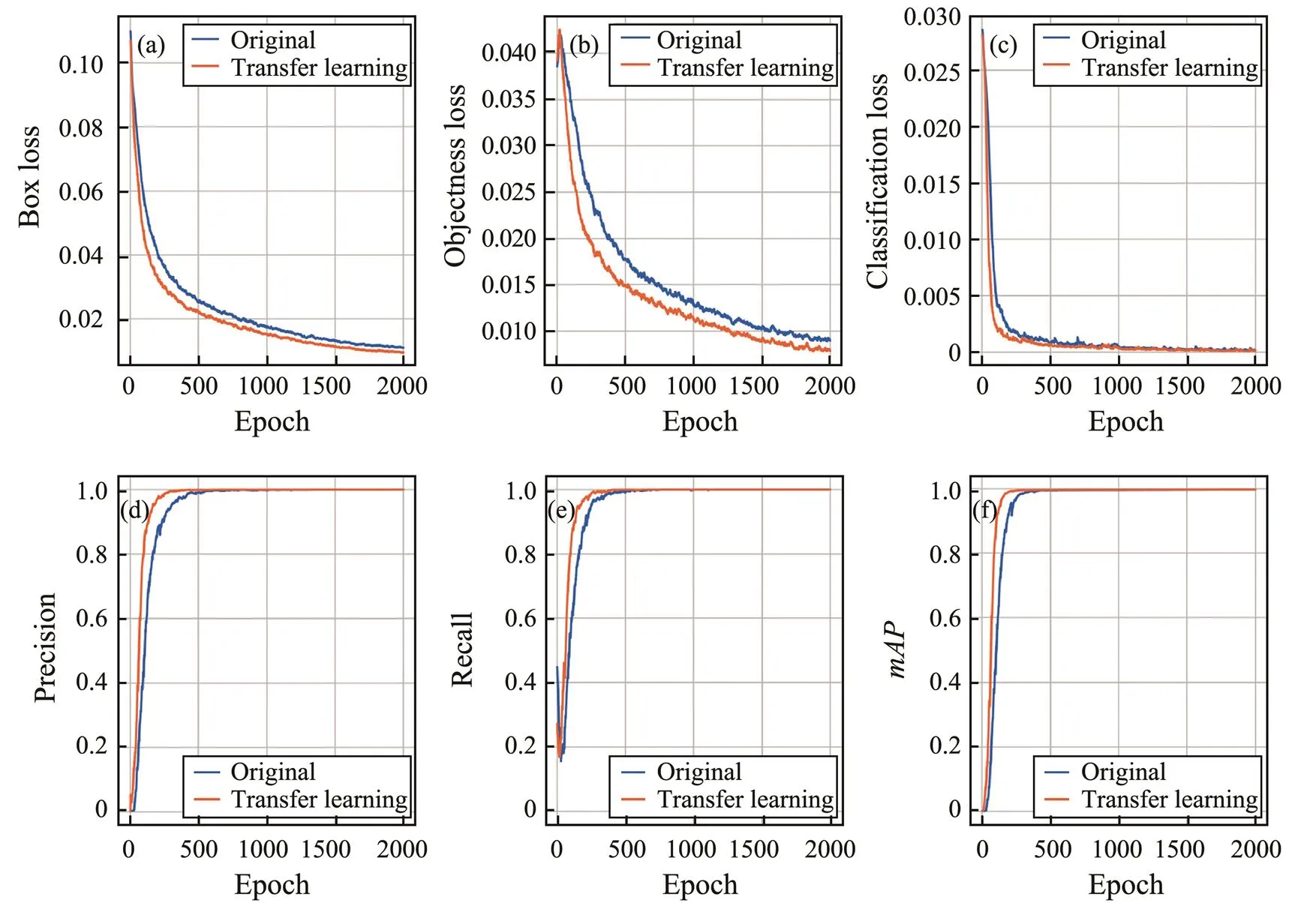
Fig.13 Variation of training and validation metrics of using transfer learning.

For comparison, under the condition of the same small dataset, Mask’s-CNN was 70%, and that of YOLO- v5 was 59.56%. However, the training period of Mask- CNN was long. The speed on the test set was 5 FPS, and the average speed of YOLOv5 was 100 fps, which enabled real-time detection.

5 Conclusions

In this paper, a real-time seabed sediment recognition model with YOLOv5 was proposed. The model can input the entire imagery without manual image cutting and feature election. It provides location information and makes real-time detection possible. This paper used datasets with different sizes, four network models, multiscale training, transfer learning, and Adam optimizer for training and vi- sually displayed and analyzed the performances of all five methods. The results showed a relatively significant performance improvement in large datasets, simple models, and the Adam optimizer. The findings provide a guiding significance for readers in selecting appropriate practice methods.

However, the proposed method has disadvantages, such as 1) low test and evaluation index values and 2) the limited generalization capability of the model. We hypothesized that these disadvantages are caused by the wide range of size variation and unclear boundary of the seabed sediment identification target. The method used in this paper still has room for further development. Our future research directions will focus on the use of a more comprehensive dataset and improving the network model structure to be suitable for the recognition of seabed sediments.

Acknowledgements

This work is funded by the Natural Science Foundation of Fujian Province (No. 2018J01063), the Project of Deep Learning Based Underwater Cultural Relics Recognization (No. 38360041), and the Project of the State Administration of Cultural Relics (No. 2018300).

Berthold, T., Leichter, A., Rosenhahn, B., Berkhahn, V., and Valerius, J., 2018. Seabed sediment classification of side-scan sonar data using convolutional neural networks.. Honolulu, 1-8.

Blondel, P., 2000. Automatic mine detection by textural analysis of COTS sidescan sonar imagery., 21 (16): 3115-3128.

Bochkovskiy, A., Wang, C.Y., and Hong, Y., 2020. YOLOv4: Op-timal speed and accuracy of object detection.:10.48550/arXiv.2004.10934.

Chik, W.B., 2008. Lord of your domain, but master of none: The need to harmonize and recalibrate the domain name regime of ownership and control., 16 (1): 8-72.

Coiras, E., Petillot, Y., and Lane, D.M., 2007. Multiresolution 3-D reconstruction from side-scan sonar images., 16 (2): 382-390.

Collier, J.S., and Humber, S.R., 2007. Time-lapse side-scan so- nar imaging of bleached coral reefs: A case study from the Seychelles., 108 (4): 339-356.

Dewi, C., Chen, R.C., and Yu, H., 2020. Weight analysis for various prohibitory sign detection and recognition using deep learning., 79 (43): 32897-32915.

Dura, E., Zhang, Y., Liao, X.J., Dobeck, G.J., and Carin, L., 2005. Active learning for detection of mine-like objects in side-scan sonar imagery., 30 (2): 360-371.

Flores, N.Y., Collas, F.P.L., Mehler, K., Schoor, M.M., Feld, C.K., and Leuven, R.S.E.W., 2021. Assessing habitat suit- ability for native and alien freshwater mussels in the River Waal (the Netherlands), using hydroacoustics and species sen- sitivity distributions., 27 (1): 187-204.

Greene, A., Rahman, A.F., Kline, R., and Rahman, M.S., 2018. Side scan sonar: A cost-efficient alternative method for measur-ing seagrass cover in shallow environments., 207: 250-258.

Gruzinov, V.M., Dyakov, N.N., Mezenceva, I.V., Malchenko, Y.A., and Korshenko, A.N., 2019. Sources of coastal water pollution near sevastopol., 59 (4): 523-532.

Kingma D., and Ba J., 2014. Adam: A method for stochastic op- timization.:10.48550/arXiv.1412.6980.

Kumar, A., Kalia, A., Verma, K., Sharma, A., and Kaushal, M., 2021. Scaling up face masks detection with YOLO on a novel dataset., 239: 166744.

Lamarche, L.G., 2011. Unsupervised fuzzy classification and ob-ject-based image analysis of multibeam data to map deep water substrates, Cook Strait, New Zealand.,31 (11): 1236-1247.

Li, S., Gu, X., Xu, X., Xu, D., Zhang, T., Liu, Z.,, 2021. Detection of concealed cracks from ground penetrating radar images based on deep learning algorithm., 273: 121949.

Lucieer, V., and Lucieer, A., 2009. Fuzzy clustering for seafloor classification., 264 (3): 230-241.

Luo, X., Qin, X., Wu, Z., Yang, F., Wang, M., and Shang, J., 2019. Sediment classification of small-size seabed acoustic images using convolutional neural networks., 7: 98331-98339.

Ma, H., Liu, Y., Ren, Y., and Yu, J., 2019. Detection of collapsed buildings in post-earthquake remote sensing images based on the improved YOLOv3., 12 (1): 44.

Microsoft, 2017. Common objects in context dataset. https://co- codataset.org/.

Ozturk, T., Talo, M., Yildirim, E.A., Baloglu, U.B., Yildirim, O., and Rajendra Acharya, U., 2020. Automated detection of CO- VID-19 cases using deep neural networks with X-ray images., 121: 103792.

Padilla, R., Netto, S.L., and Silva, E., 2020. A survey on perfor- mance metrics for object-detection algorithms.. Niteroi, 237-242.

Qin, X., Luo, X., Wu, Z., and Shang, J., 2021. Optimizing the sediment classification of small side-scan sonar images based on deep learning., 9: 29416-29428.

Ren, S., He, K., Girshick, R., and Sun, J., 2017. Faster R-CNN: Towards real-time object detection with region proposal net- works., 39 (6): 1137-1149.

Sun, C., Hu, Y., and Shi, P., 2020. Probabilistic neural network based seabed sediment recognition method for side-scan sonar imagery., 410: 105792.

Sun, C., Wang, L., Wang, N., and Jin, S., 2021. Image recognition technology in texture identification of marine sediment sonar image., 2021 (2): 1-8.

Sutskever, I., Martens, J., Dahl, G., and Hinton, G., 2013. On the importance of initialization and momentum in deep learning.Atlanta, Georgia, USA, 2176-2184.

Uchimoto, K., Nishimura, M., Watanabe, Y., and Xue, Z., 2020. An experiment revealing the ability of a side-scan sonar to detect CO2bubbles in shallow seas., 10 (3): 591-603.

Ultralytics, 2020. YOLOv5. https://github.com/ultralytics/YOLO- v5.

Wang, X., Zhao, J.H., Zhu, B.Y., Jiang, T.C., and Qin, T.T., 2018. A side scan sonar image target detection algorithm based on a neutrosophic set and diffusion maps., 10 (2): 295.

Xi, H.Y., Wan, L., Sheng, M.W., Li, Y.M., and Liu, T., 2017. The study of the seabed side-scan acoustic images recognition using BP neural network. In:.Chen, G.,., eds., Springer, Sin- gapore, 130-141.

Yan, J., Meng, J., and Zhao, J., 2021. Bottom detection from backscatter data of conventional side scan sonars through 1D-UNet., 13 (5): 1-23.

Yu, Y., Zhao, J., Gong, Q., Huang, C., Zheng, G., and Ma, J., 2021. Real-time underwater maritime object detection in side- scan sonar images based on transformer-YOLOv5.,13 (18): 3555.

Yulin, T., Jin, S., Bian, G., and Zhang, Y., 2020. Shipwreck target recognition in side-scan sonar images by improved YOLOv3 Model based on transfer learning., 8: 173450-173460.

Zhu, Z., Cui, X., Zhang, K., Ai, B., Shi, B., and Yang, F., 2021. DNN-based seabed classification using differently weighted MBES multifeatures., 438: 106519.

Zhuang, F., Qi, Z., Duan, K., Xi, D., Zhu, Y., Zhu, H.,, 2021. A comprehensive survey on transfer learning., 109 (1): 43-76.

(May 8, 2022;

September 21, 2022;

October 21, 2022)

© Ocean University of China, Science Press and Springer-Verlag GmbH Germany 2023

. E-mail: pshi@ustb.edu.cn

(Edited by Chen Wenwen)