Parameterization Method of Wind Drift Factor Based on Deep Learning in the Oil Spill Model

YU Fangjie, GU Feiyang, ZHAO Yang, HU Huimin, ZHANG Xiaodong,ZHUANG Zhiyuan, and CHEN Ge

Parameterization Method of Wind Drift Factor Based on Deep Learning in the Oil Spill Model

YU Fangjie1), 2), GU Feiyang1), ZHAO Yang3), *, HU Huimin1), ZHANG Xiaodong4),ZHUANG Zhiyuan1), and CHEN Ge1), 2)

1),,,266100,2), Laoshan Laboratory,266100,3),,,266100,4),266100,

Oil spill prediction is critical for reducing the detrimental impact of oil spills on marine ecosystems, and the wind strong- ly influences the performance of oil spill models. However, the wind drift factor is assumed to be constant or parameterized by linear regression and other methods in existing studies, which may limit the accuracy of the oil spill simulation. A parameterization method for wind drift factor (PMOWDF) based on deep learning, which can effectively extract the time-varying characteristics on a regional scale, is proposed in this paper. The method was adopted to forecast the oil spill in the East China Sea. The discrepancies between predicted positions and actual measurement locations of the drifters are obtained using seasonal statistical analysis. Results reveal that PMOWDF can improve the accuracy of oil spill simulation compared with the traditional method. Furthermore, the parameteriza- tion method is validated with satellite observations of the Sanchi oil spill in 2018.

oil spill prediction; deep learning; wind drift factor; regional parameterization; East China Sea

1 Introduction

The East China Sea is approximately 770000 square ki- lometers, adjacent to the South China Sea and the Yellow Sea, and linked to the Japan Sea by the Tsushima Strait (Ta- kahashi and Morimoto, 2013). This area has abundant oil and natural gas resources, with roughly 14.4 million tons of technically recoverable reserves in total. With the de-velopment of oil drilling and transportation, the probabi-lity of unexpected oil spill accidents appears to be increas- ing substantially. As demonstrated by the Penglai 19-3 oil platform spill accident and the oil transport accident caused by the collision between the Panama-registered oil tanker Sanchi and the Chinese bulk carrier Crystal, marine oil spill disasters are destructive to marine ecology and economic development (Guo., 2012; Zhang., 2020). The East China Sea area has a complex geological structure,and its oil platforms are far away from the mainland, whichmay introduce challenges to the emergency treatment ofthe oil spill (Xu., 2020). Therefore, an accurate oil spillforecast system applicable to the East China Sea is required to plan emergency response management decisions to re-duce the negative impact of oil spills and protect the en- vironment.

In recent years, various numerical models have been wide-ly used to simulate the transport and the fate of oil spills and are applied in practical oil spill events worldwide, such as OSCAR (oil spill contingency and response model) (Reed., 1995), GNOME (General NOAA Operational Mo- deling Environment) (Zelenke., 2012), the OSIS sys- tem (Leech., 1993), the 3D Oil Spill Model and Re- sponse System OILMAP (Spaulding., 1994), and ME- DSLICK-II for short-term oil spill forecasting (De Domi- nicis., 2013), have been developed. Oil spill models can be divided into Eulerian and Lagrangian methods. In general, practical Eulerian formulas can easily represent the complex and nonlinear transformation process affected by environmental parameters (Guo and Wang, 2009). By con-trast, Lagrangian models are convenient, efficient, cost-ef- fective, and suitable for simulating the advection process influenced by wind and current (Keramea., 2021). Therefore, the Eulerian-Lagrangian method can be used to calculate the oil weathering process in fixed grids and the oil transport process in a particle-tracking frame (Yu., 2016). The wind is considered the main influential com- ponent in the oil slick movement (Kabdasli., 2010; Li., 2013; Khade., 2017). Wind drift is the ef- fect of wind on the oil slick on the sea surface, which moves oil at a specific proportion of the wind speed and at a cer- tain angle to the wind direction (Lardner and Zodiatis, 2017; Li., 2019). In most oil spill models, the wind drift fac- tor usually takes an empirical value (Abascal., 2009). This empirical parameter represents average conditions andis regarded as one of the primary contributors to uncertain-ty in the oil spill model (Hodges., 2015; Zodiatis., 2017; Guo., 2018). The changes in complex environ- mental conditions, such as water depth characteristics and meteorological circumstances, determine that the wind driftfactor should not be a constant. Kampouris. (2021) performed simulations for different seasons to investigate the atmospheric forcing uncertainties, particularly the in- tensity and direction of the wind, on the oil spill model. Gautama. (2016) estimated the best leakage parame- ters of the oil spill through the assimilation of SAR obser- vations into a 2D Lagrangian trajectory model. Some re- searchers adopted a trial-and-error procedure using satel- lite imagery to validate the different wind drift factors in the oil spill model (Kim., 2014; Pan., 2020). Yu. (2020) employed linear regression combined withoceanographic and drifter data to obtain a wind drift factor in a year suitable for the studied area.

The above studies reveal that the investigations on wind drift factor have experienced the process from empirical va- lue to linear method. However, these approaches are inade- quate for identifying the nonlinear features of spatial and temporal variations in different regions. To deal with this issue and increase the accuracy of the oil spill prediction, a parameterization method of wind drift factor (PMOWDF) based on deep learning, which can directly extract the re- gional features from the training data without any prior knowledge, is proposed in this paper. Moreover, the me- thod is adopted into the Eulerian-Lagrangian equation to establish an accurate oil spill model in the East China Sea. The observations of satellites cannot cover all possible sce- narios, and drifters can be carried with oil for days; thus, the datasets of drifter trajectories are employed to evalu- ate the model (Onay., 2020; Yu., 2020; Zhu., 2021). The results are also subjected to statistical analysis on a seasonal basis. Furthermore, the PMOWDF is vali-dated using satellite observations of the Sanchi oil spill ac- cident in 2018.

This paper is organized as follows. The datasets are pre- sented in Section 2. The PMOWDF and the oil spill mo- del, including the oil slick motion formulas, are described in Section 3. The optimized wind drift factor and the pre- dicted oil spill trajectory are illustrated in Section 4. The validation of the oil spill model and the significance of windparameter correction are discussed in Section 5. Finally, the conclusions of this research are described in Section 6.

2 Data

2.1 Oil Spill Model

Predicting the trajectory of the spilled oil is usually achi- eved by numerical models. This paper uses a regional mo- del based on the i4OilSpill model, which employs the Eu- lerian-Lagrangian approach to simulate the oil transport and fate by dividing the water body into several horizontal lay- ers (Yu., 2016). Existing studies have demonstrated the effectiveness of this model in the Bohai Sea and the South China Sea (Yu., 2018, 2020). The model requires input data, such as the initial position of the oil slick, the time, duration, and coverage of the oil spill, the type of oil, and wind and sea current data.

2.2 Drifters

Drifters (surface drifting buoys) are designed to be tran-sported by ocean currents and are used to study surface cir- culation and oceanographic dynamics. These characteris- tics increase their usefulness for the validation of Lagran- gian particle models and can be considered oil spill tracers (De Dominicis., 2016). The drifter dataset used in thisstudy, which includes hourly geographical locations and ho-rizontal velocities along drifter trajectories, is from the Na- tional Oceanic and Atmospheric Administration (NOAA) Atlantic Oceanographic and Meteorological Laboratory (https://www.aoml.noaa.gov/phod/gdp/hourly_data.php) (Elipot., 2016). Drifter data within the range of the East China Sea (23˚–33˚N, 117˚–131˚E) from 2010 to 2015,including drifter ID, deployment time, the latitude and longi- tude of the first record, and hourly geographical locations and horizontal velocities along trajectories, are acquired. Thedata from 2010 to 2014 are used to calculate parameter cor- rections, and the data from 2015 are used for statistical va- lidation. The trajectories of the drifters passing through the East China Sea in 2015 are illustrated in Fig.1.

2.3 Oceanographic Data

Real-time wind and current forecasts, typically provided by supportive environmental models, are required for a re- liable oil spill forecast (Spaulding, 2017; Pan., 2021). The ocean wind data applied in this research are from the ECMWF (European Centre for Medium-Weather Forecast-ing) ERA-Interim reanalysis data (https://www.ecmwf.int/ en/forecasts/datasets). The parameter of a 10mwind component and a 10mwind component was selected, with a spatial resolution of 0.125˚ and a temporal resolu- tion of one day. The surface current data are modeled em- ploying HYCOM (hybrid coordinate ocean model) (https:// www.hycom.org), which includes tidal forcing, with the grids of 0.08˚ latitude × 0.08˚ longitude and a time resolu- tion of 6h. The system uses a 3D variational scheme and assimilates available satellite altimeter observations, satel- lite, andsea surface temperature, as well asvertical temperature and salinity profiles from XBTs, Ar- go floats, and moored buoys (Cummings and Smedstad, 2013). Astronomical tidal potential forcing for eight com- ponents (M2, S2, K1, O1, N2, P1, K2, and Q1) was imple-mented in HYCOM forced by the National Centers for En- vironmental Prediction Climate Forecast System Version 2 (CFSv2).The boundary forcing adopts the Flather condi- tion, wherein the eight largest components are specified as complex amplitudes at each boundary point. The tidal si- mulation employs tidal self-attraction and loading and al- lows for a curvilinear grid with nodal corrections. Exist- ing studies have shown the accuracy of global HYCOM tidal elevations and currents at a resolution of 0.08˚(Ar- bic, 2010; Timko, 2019). The feasibility of uti- lizing the current data with a resolution of 0.08˚ for oil spillsimulation in the East China Sea has also been demonstrated by existing studies (Pan, 2020; Yang, 2021). In addition, Fig.1 shows that most drifters utilized for the cur- rent study were located some distance from the shore; thus, the tidal forcing is relatively weak. Therefore, the current data from HYCOM with a horizontal resolution of 0.08˚ can support the oil spill simulation in this research. The wind and current data were obtained from 2010 to 2015 within the scope of the East China Sea (23˚–33˚N, 117˚–131˚E). Furthermore, the wind and current data in January 2018 with the scope of the East China Sea were obtained for the Sanchi oil spill simulation.

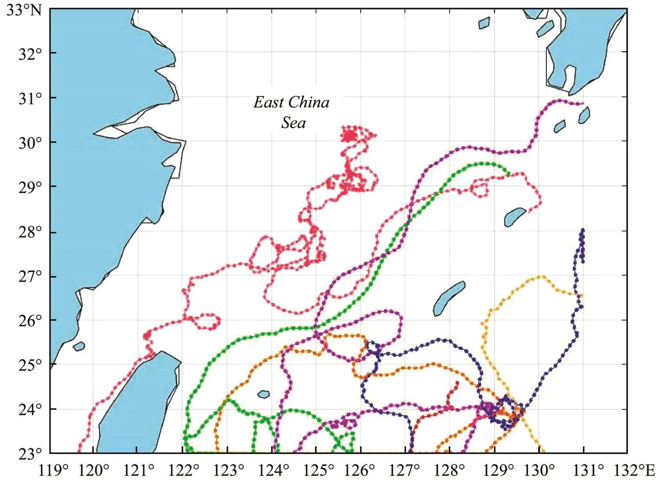
Fig.1 Trajectories of drifters appeared in the East China Sea in 2015.

3 Methods

The oil spill forecasting framework and the related me- thods are formally introduced in this section. Fig.2 shows the structure of the oil spill forecasting system, which com- prises the following two parts: optimizing the wind drift fac- tor by introducing the deep learning algorithm and conduct- ing oil spill simulation using the Eulerian-Lagrangian oil spill model.

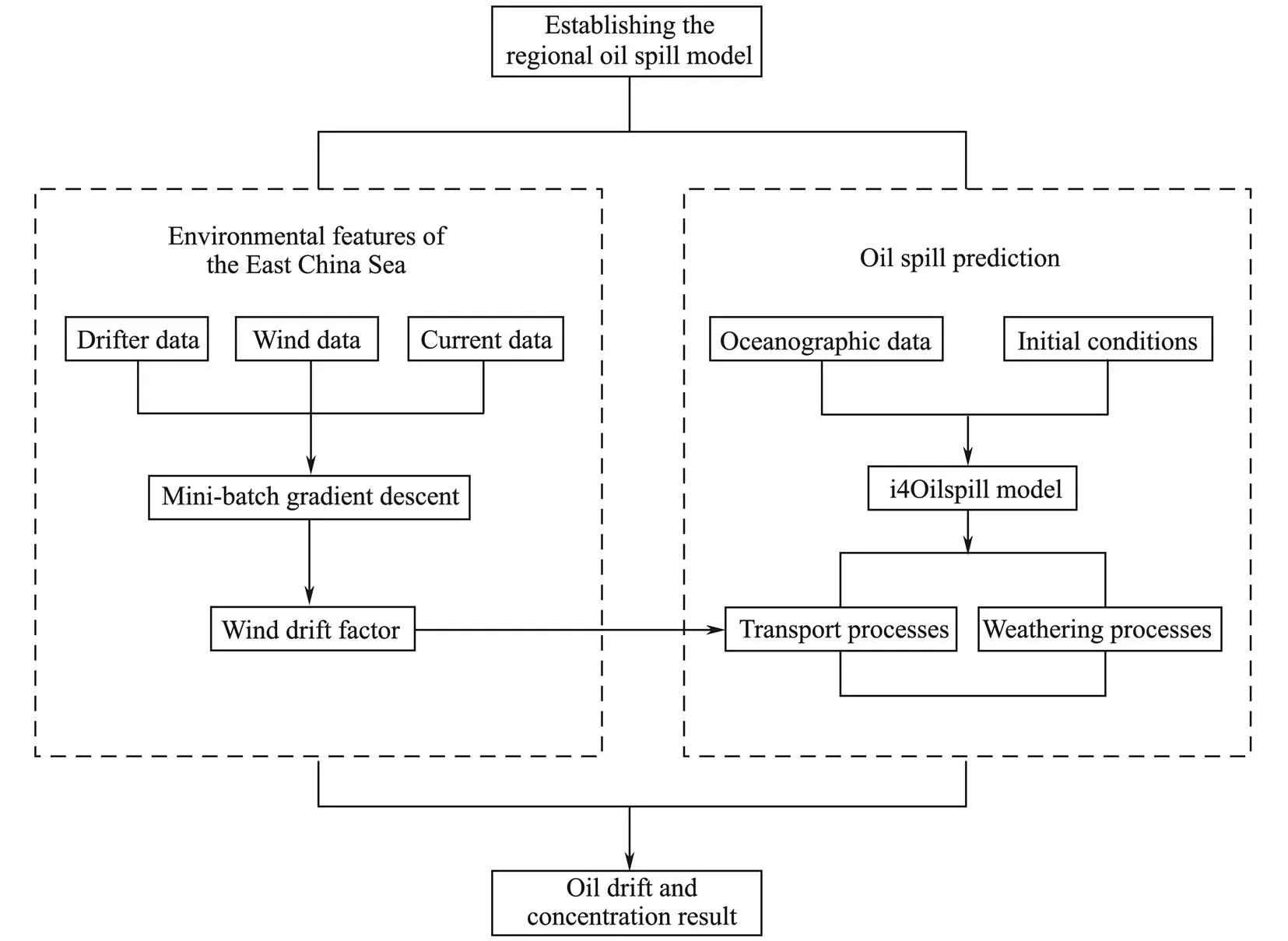
Fig.2 Structure of the oil spill forecasting system.

3.1 Oil Spill Simulation

In the Eulerian-Lagrangian oil spill model, the transport process of oil particles in the marine environment is ge-nerally attributed to advection by the large-scale flow field, with dispersion driven by turbulent flow components. More- over, the concentration of the oil changes due to multiple physical and chemical processes known as the weathering processes. The general equation for the concentration of an oil tracer in the marine environment is as follows.

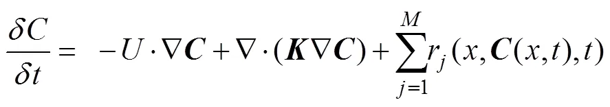
The current study focused on the transport process of oil particles on the sea surface here. This process can be ex- pressed as follows:

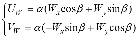
whereWandWdenote the wind speed at 10m above the sea surface in theanddirections, respectively;is call- ed the wind drift factor, wherein a spatially and temporal- ly fixed constant of 3% is used in most oil spill models;indicates the drift angle. However, a general assumption is that the wind drift factor varies with the sea state conditionsand plays an important role in the oil spill simulation (Lehr and Simecek-Beatty, 2000; Yu., 2016). Herein, thePMOWDF model, which can reflect the time-varying cha- racteristics precisely and simulate the transport of the oil spill accurately, is proposed. Furthermore, deep learning is merged with the proposed model to realize a thorough in- quiry into the calculation of the variable wind drift factor. The following sections will present how the method works.

3.2 PMOWDF Based on Deep Learning

This subsection describes the basic theory of the mini- batch gradient descent (MBGD) adopted in the model to calculate the wind drift factor. MBGD is an extension of gradient descent, a classic and robust parameter optimiza- tion algorithm (Khirirat., 2017). The main idea of the algorithm is to update parameters with ‘batch_size’ samples during each iteration process, wherein the batch_size re- presents the divided magnitude of the sample and deter- mines the direction of the optimization. This approach can effectively reduce the highly time-consuming and compu- tationally complex gradient algorithm. Furthermore, such an approach allows for considerable flexibility in select- ing data samples and increases data utilization efficiency.

The position and velocity of the drifters deployed in the East China Sea are employed in the current study to rep- resent the oil spill trajectory. The entire process for the MBGD application to obtain the wind drift factor is present- ed in Fig.3 and is divided into the following three parts: constructing the oil spill dataset by combining the ocean cur- rent, wind, and drifter data; training the parameter optimi- zation model; and testing the parameter optimization mo- del. The data from 2010 to 2014 are employed as the train- ing dataset to calculate the best wind drift factor, while those from 2015 are used as the testing dataset for statisti- cal validation.

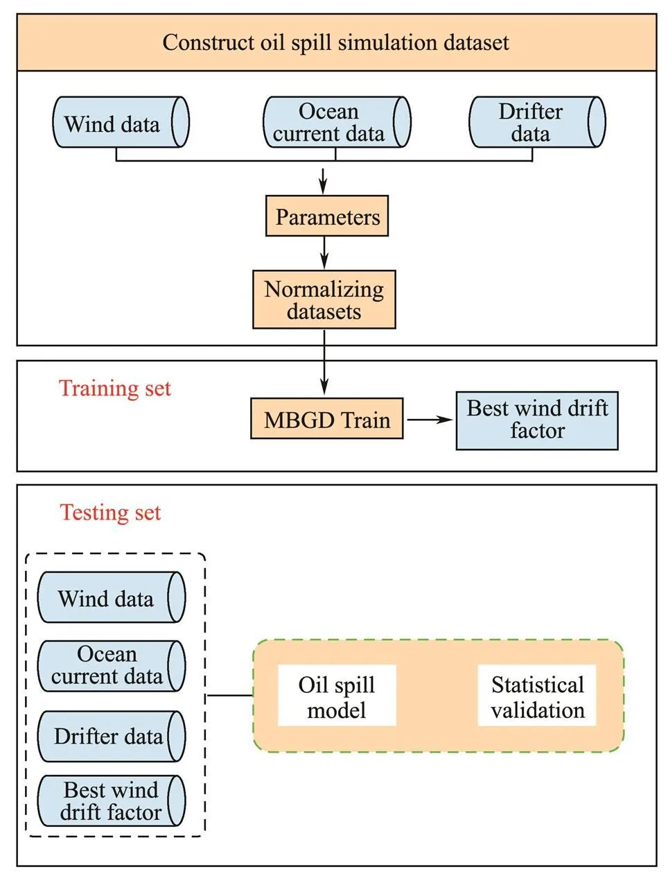
Fig.3 Entire process of applying MBGD to obtain the best wind drift factor.

3.2.1 Constructing the oil spill dataset

The oil spill transport process on the sea surface is de-scribed as the dataset={(i),(i)}, where(i)={(i),(i)}denotes the wind and current fields and(i)represents the movement trajectory of the drifter, which can be consid- ered oil spill tracers.

3.2.2 Parameter optimization model creation and initialization

The model creation comprises the backpropagation net- work establishment and the MBGD optimization, wherein the backpropagation network maps input values to output values, and the MBGD optimizes the weights (wind drift factor), respectively. The network in the current study com- prises two input nodes: a hidden layer and an output layer. The initial parameters of the MBGD are shown in Table 1.

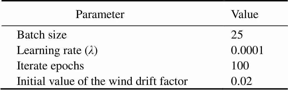
Table 1 Parameters of the MBGD

3.2.3 Parameter optimization model training

The algorithm aims to establish a cost function between the predicted position and the measured location of drifters and minimize the cost function by iteratively updating the initial wind drift factor to find the best value. Fig.4 shows the process of the wind drift factor optimization using the MBGD: Fig.4(a) presents the basic principle of iterative optimization through updating the wind drift factor in de- termining which one can obtain the minimum value of cost function, and Fig.4(b) presents the convergency of iterative optimization. The constructed cost function is shown as fol- lows:

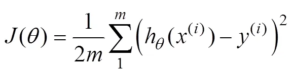
whereh((i)) is the dot product of the input wind and current speed with the parameter, representing the predict- ed displacement of drifters,indicates the number of sam- ples, andis the wind drifter factor. The parameters are iteratively updated, and the batch size is added on the ba- sis of the gradient descent algorithm. The resulting formu- la is as follows:

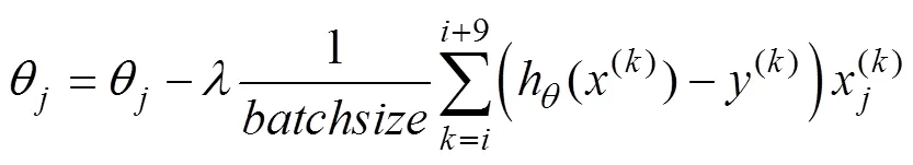
whereis expressed as the amount of sample da- ta used for each iteration update,represents the number of data, andsignifies the learning rate. The optimal wind drift factor can be obtained from the above equations.

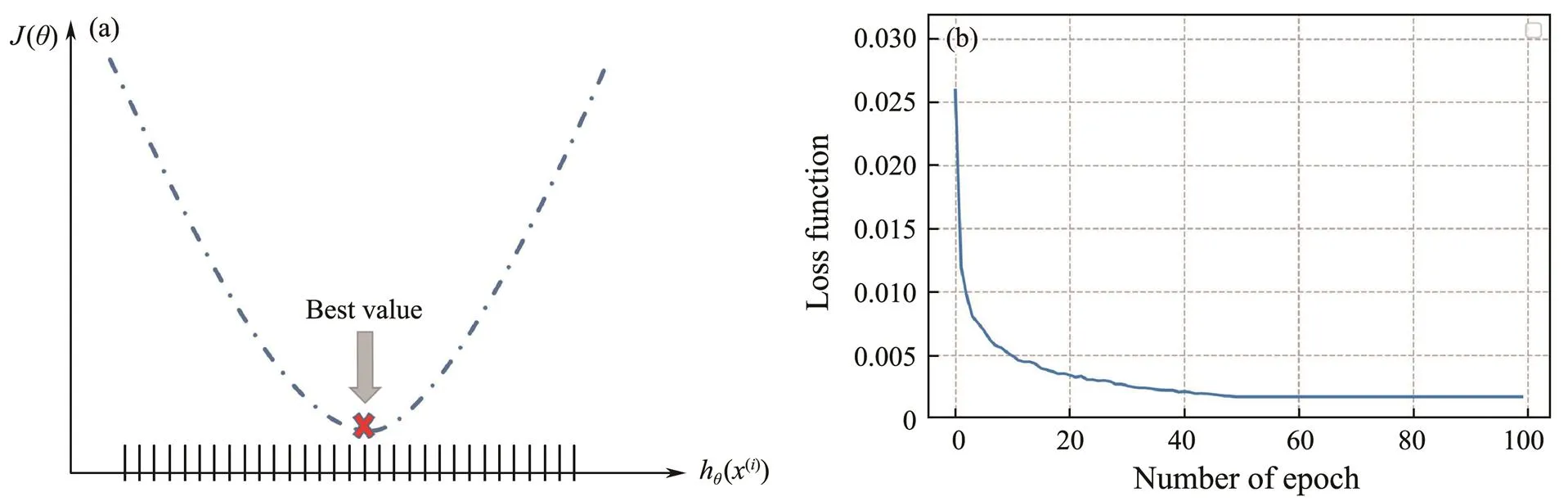
Fig.4 Schematic of wind drift factor optimization using MBGD. (a) Basic principle of iterative optimization, where the red symbol represents the best parameter. (b) Convergency of the MBGD during the optimization of the wind drift factor.

3.2.4 Parameter optimization model testing

After the initialization and training of the parameter op- timization model, the best wind drift factors are combined with the oil spill model to construct the statistical valida- tion.

4 Results

4.1 Wind Drift Factor Calculation

Based on the parameter optimization model derived above, the wind drift factor optimization for the East China Sea area was explored using the drifter data combined with high-resolution wind and current data from 2010 to 2014. The wind and current data are set as inputs, while drifterdata are set as outputs. The dataset was divided into 12 parts by month, and the mapping network was established from input to output value, respectively. The optimal wind drift factors are updated during the iteration process of the MBGD, and the final results are shown in Table 2.

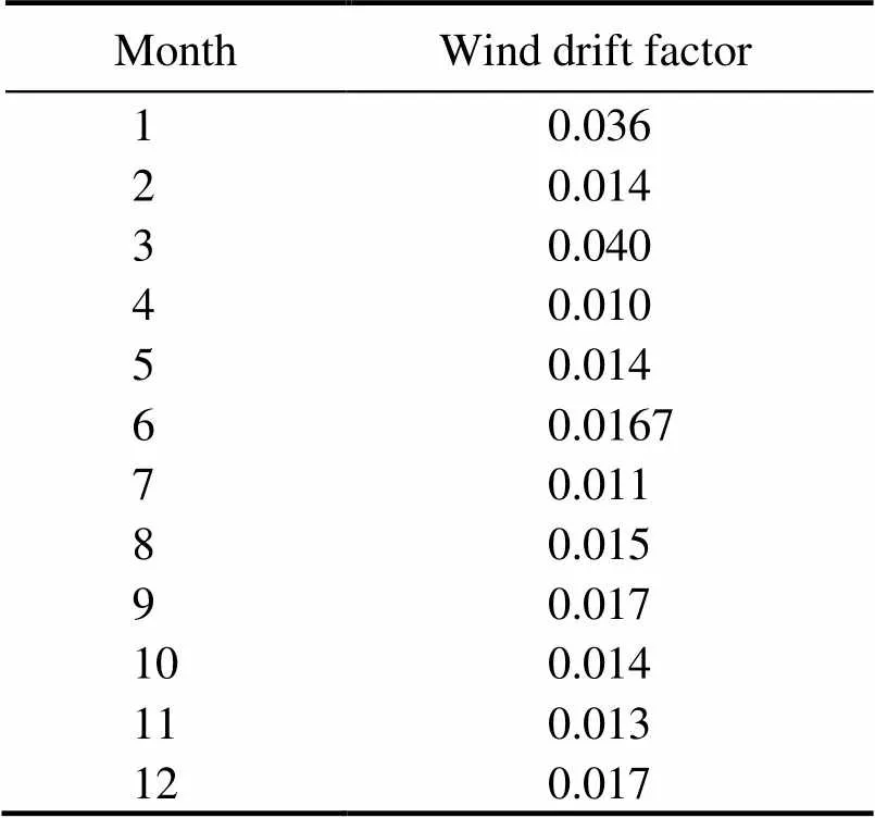
Table 2 Wind drift factor for each month in the East China Sea

The wind drift factor, parameterized by deep learning, evolves over time. These optimized values are adopted in- to the oil spill model to forecast the oil spill trajectory. Fur- thermore, the results using the optimized wind drift factor are compared with those using the empirical value.

4.2 Oil Spill Track Simulation

The applicability of the PMOWDF in oil spill prediction is investigated using drifters. Drifter data in the East China Sea from January 1, 2015 to December 25, 2015, totaling 286, are chosen for successive calculations and validations. The drifter data provide the initial conditions of the oil spill simulation; these data, coupled with oceanographic data, are then input into the original empirical parameter model and the model optimized by PMOWDF. Each simulation lasted for 72h and had an hourly time resolution. The ma- rine environment of each quarter contains similar charac- teristics. Therefore, one simulation result was randomly chosen from each quarter as an expression, with starting dates of January 5, April 8, July 14, and November 17 (Fig.5).

The color bar in the figure represents the oil spill con- centration (tkm−²). The simulation results of the originalmodel are shown in green, while those of the model opti- mized by the PMOWDF are displayed in blue for compari- son. The red star-shaped points in the figure indicate the actual measured position of the drifter corresponding to the simulation duration.

The oil spill concentration ranges between 0.15 and 0.5tkm−2, with an average value of approximately 0.25tkm−2. The oil slick has a high intermediate and low edge con-centration because it spreads from the middle to the edge. At short oil spill durations, the difference between the si-mulation results of the two models is insignificant. Asthe oil spill simulation time increases, the oil spill area will spread out, and the contaminated area will increase. In ad- dition, the concentration and the moving direction of the oil spill are related to local climate conditions due to changesin the marine environment, such as wind speed, wind direc- tion, current velocity, and sea temperature.

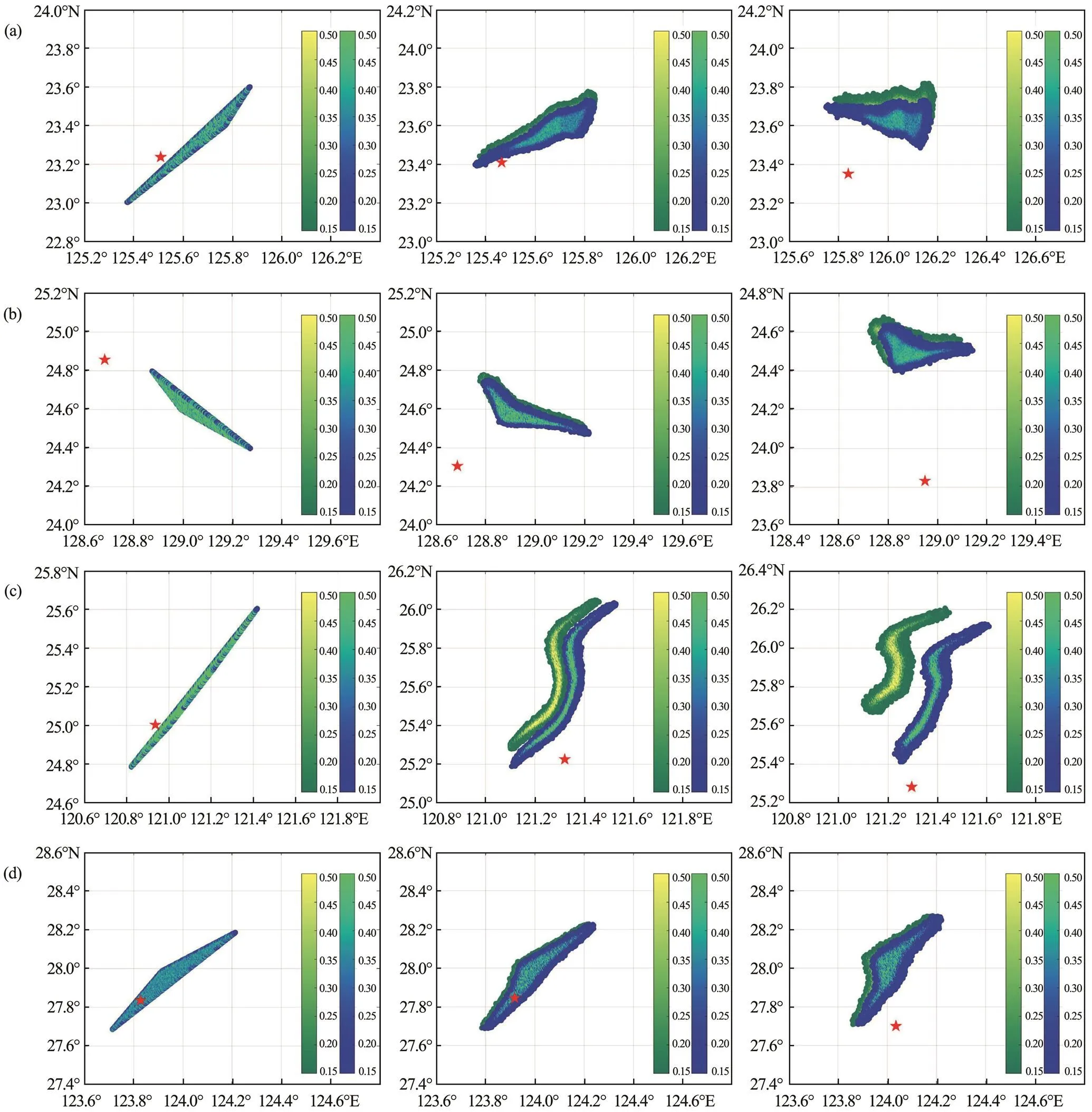
Fig.5 Simulation of oil concentrations (tkm−2) and the trajectories with durations of 24, 36, and 72h from left to right. (a), January 5 (winter); (b), April 8 (spring); (c), July 14 (summer); (d), November 17 (autumn).

The fate processes of the oil spill are illustrated in Fig.6. Consistent with the oil spill trajectory in Fig.5, the oil wea-thering processes with starting dates of January 5, April 8, July 14, and November 17 are selected for demonstration. The evaporation process of the oil showssimilarity at diffe- rent times. The fraction of evaporation rapidly increases in the first few hours of the oil spill simulation and then re- mains stable at a value of approximately 30%. Meanwhile,the fraction of emulsification increases with the simulation duration and stabilizes after some time. In the four oil spill simulations, the final emulsification ratesare equal, but the times at which they reach stability are different. The percen- tages of dispersed oil remain at zero at the beginning and start to increase continuously with time after 25h. Disper- sion process curves in the four simulations have different increase rates.

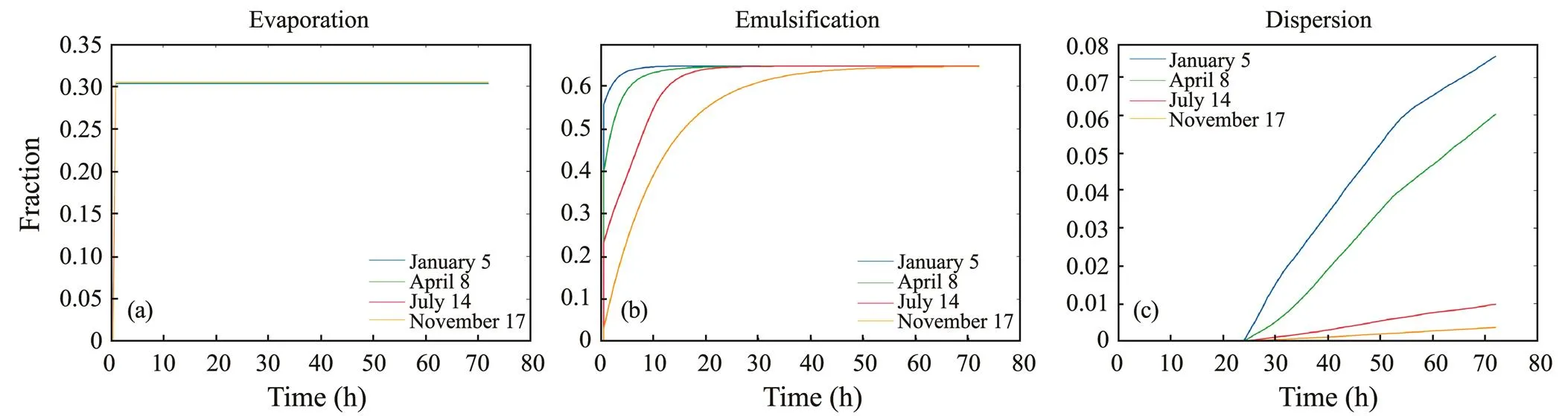
Fig.6 Oil fate processes of the oil spill in the East China Sea. (a), evaporation; (b), emulsification; and (c), dispersion.

5 Discussion

5.1 Statistical Verification of Oil Spill Drift Results in the East China Sea

The visualization of the oil spill trajectory simulation in the previous chapter (Fig.5) reveals differences in the oil spill trajectories calculated by the optimized wind drift fac- tor and the empirical value. Mean absolute error () and root mean square error () are employed to evaluate the offset between the predicted and the observed values, respectively, allowing for an accurate analysis. Their sta- tistical applications are elaborated on below.

5.1.1 Mean absolute error ()

indicates the average value of the distance be- tween the predicted and actual values of each simulation in a month, as calculated by Eq. (6).

whererepresents the number of simulation experiments conducted this month, and Δdenotes the distance between the simulated oil slick and the corresponding drifter mea- sured position. Theof the oil spill model optimized by deep learning and the original model is calculated se- parately for simulation durations of 24, 36, 48, 60, and 72h(Fig.7). The dotted lines depict the situation of the opti- mized model, whereas the solid lines represent the situa- tion where traditional empirical parameters are applied.

The mean absolute error is under 15, 20, 28, 35, and 48 km for simulated oil spill durations of 24, 36, 48, 60, and 72h, respectively. Furthermore, the error of the oil spill mo- del improved by the PMOWDF is almost always less than that of the original model at all months and five kinds of duration.

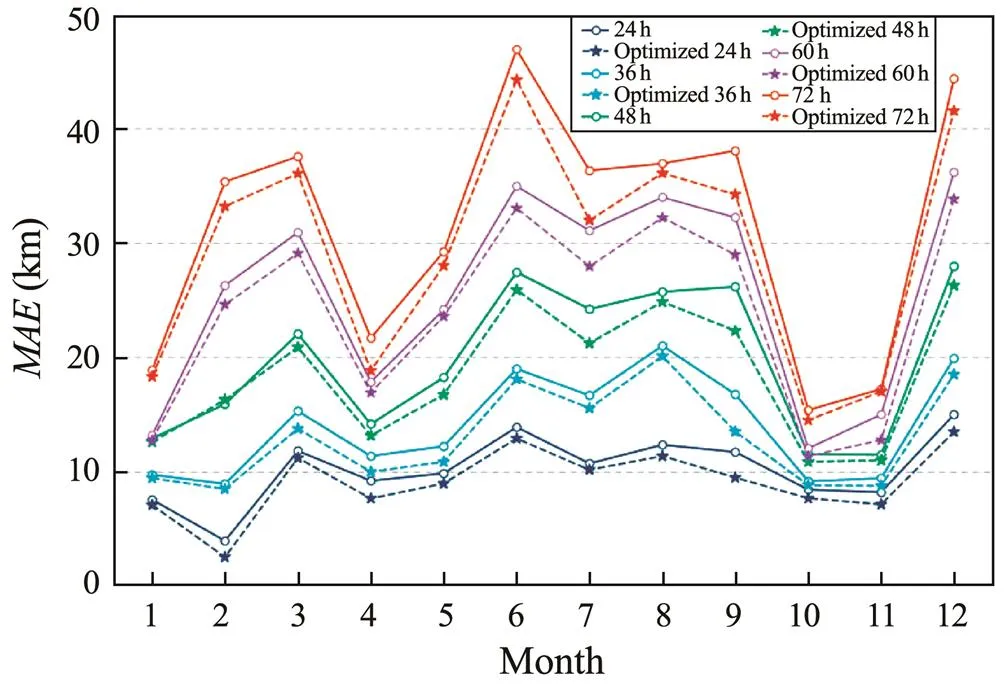
Fig.7 Mean absolute error of the two oil spill models for each month in 2015.

5.1.2 Root mean square error ()

is also used to evaluate the deviation between the predicted and measured values, as calculated by Eq. (7).

Similarly,represents the number of simulation expe- riments conducted in a month, and Δdenotes the distancebetween the predicted oil position and the corresponding measured position of the drifter.is calculated from the simulation results by using the original oil spill model. By contrast,is computed from the simulation results of the oil spill model improved by the PMOWDF (Table 3).

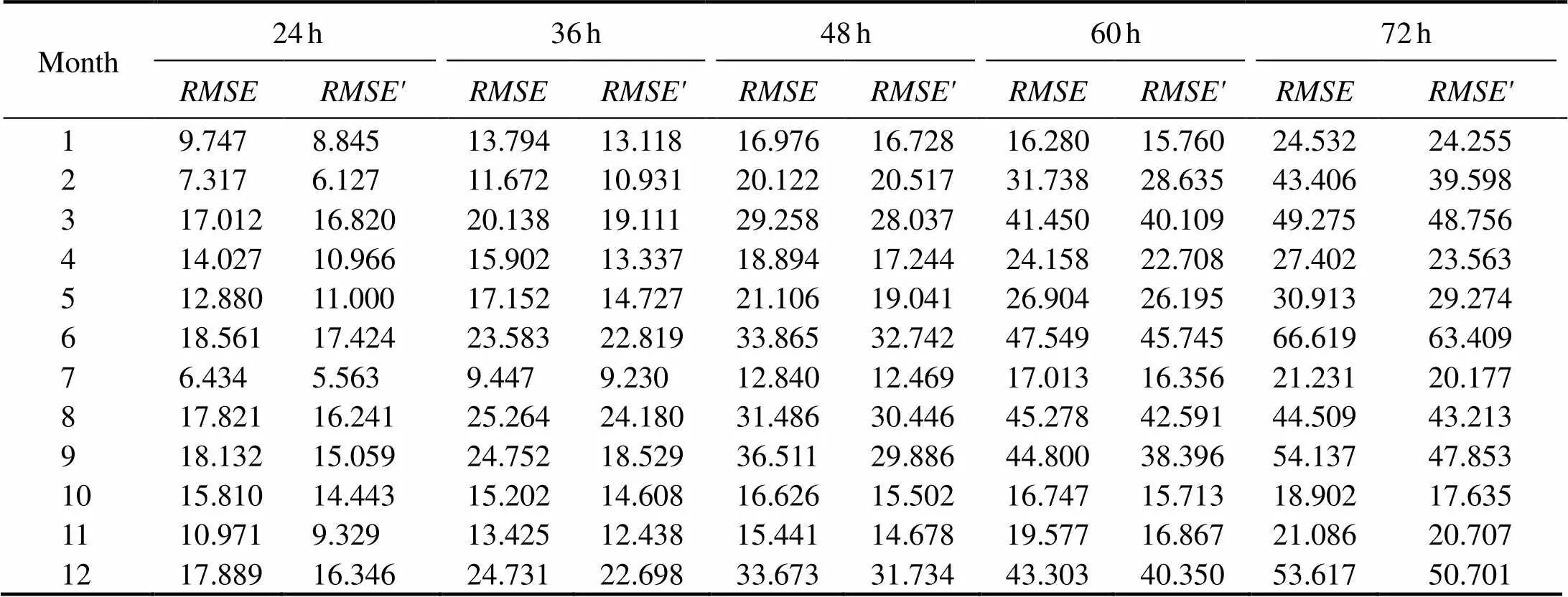
Table 3 Root mean square error of two models for a certain simulation duration

Some information can be obtained from the table. First, under the same time conditions, theis generally smaller than the, implying that the oil spill predict- tion of the model improved by the PMOWDF is more ac- curate than the original model. Second, the root mean square error gradually increases as the duration of the oil spill si- mulation rises, indicating that the simulation is accurate and the recycling of contaminants is efficient at the start of oil spill accidents. Finally, the root mean square error variesby month, indicating that the accuracy of oil spill predictioncan be affected by the local weather, such as cyclones, cold snaps, and intense typhoons.

5.1.3 Improved accuracy of the PMOWDF

The results of the previous sections show that the accu- racy of oil spill simulation can be improved by correcting the parameters in the oil spill model through deep learn- ing. To reflect the optimization degree of the PMOWDF, a functionis introduced for improved accuracy:

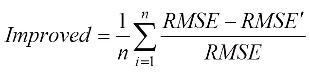
wheretakes the value of 12 in this experiment, represent- ing the number of months.andare obtained in the previous subsection, corresponding to the original and optimized models, respectively. Table 4 shows that the ac- curacy of the oil spill model increases by approximately 5.81% to 11.06%.

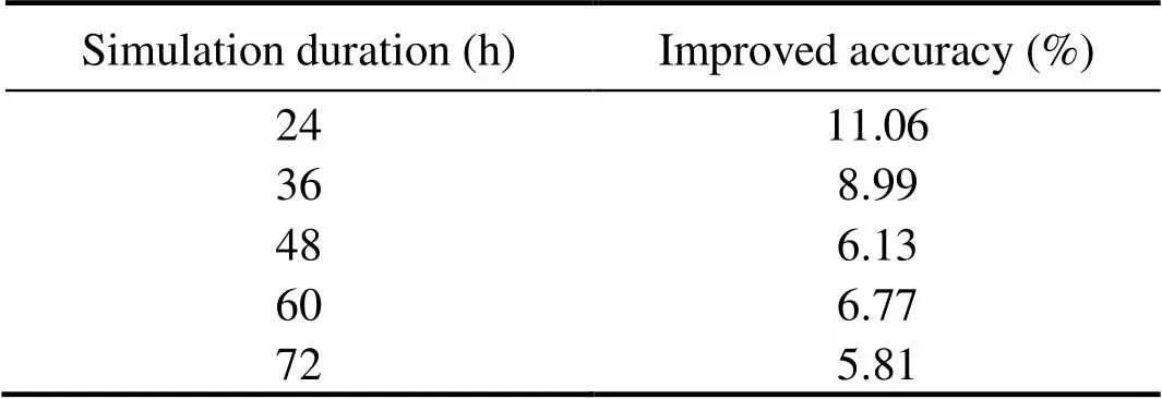
Table 4 Improved accuracy in varied duration

5.2 Seasonal Analysis of the Oil Spill Drift

The oil spill trajectory in the East China Sea is impact- ed by ocean currents, monsoons, typhoons, and seasonal variations. Therefore, further seasonal analysis is conduct- ed on the basis of the experimental results presented above. The wind drift factor,,, and the rate of accu- racy improvement of four seasons are compared using the average of three months as the value of a season (shown in Figs.8 and 9).

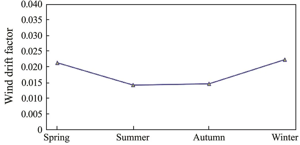
Fig.8 Mean wind drift factor suitable for the oil spill pre- diction in four seasons.

Fig.9 Mean absolute error, root mean square error, and the improved accuracy of the oil spill model optimized by deep learning in four seasons.

5.3 Validation of the Oil Spill Model by Actual Oil Spill Accidents

The PMOWDF is utilized to simulate the oil spill tra- jectory during the Sanchi collision accident in 2018, East China Sea, to further verify its applicability. Meanwhile, the linear regression method is based on Yu. (2020), and traditional empirical parameters are introduced as contrast experiments. Information regarding the Sanchi oil spill wasobtained from Pan. (2020). The distributions of the oil slicks are derived from satellite observations at 06:19 on January 15, 04:51 on January 16, and 17:42 on January 17. The data from January 15 provide the initial conditions of the simulation; they were coupled with oceanographic data and then input into three models to predict the oil slick on January 16 and 17. The time resolution of the oil spill mo- del is one hour; therefore, the simulation duration is set as 23 and 59. The detailed parameters of the model are shown in Table 5.

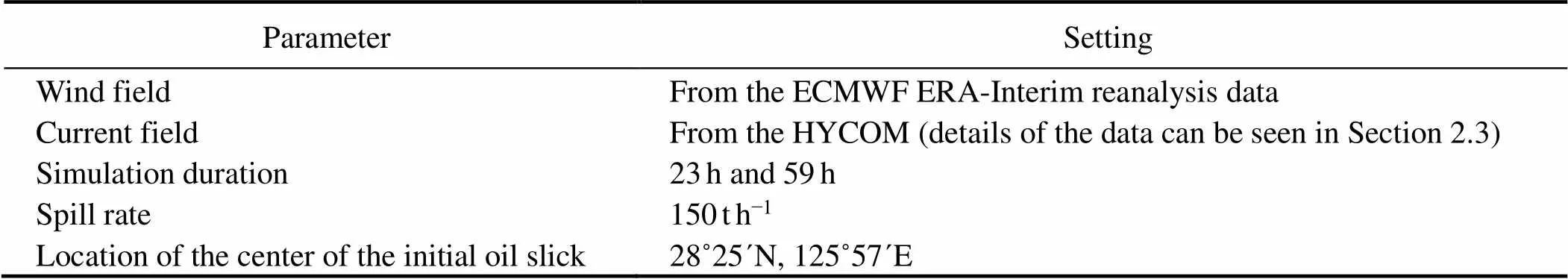
Table 5 Model settings for Sanchi oil spill simulation

Fig.10 depicts the simulation results of the oil spill mo- del optimized by the PMOWDF, the model corrected by linear regression, and the original model. The oil fate pro- cesses of the Sanchi oil spill are illustrated in Fig.11. Ta- ble 6 shows that the accuracy of the results is evaluated us-ing a percent area metric of the forecast slick area in thespill observation area. The accuracy of the simulation last- ing 23h is superior to that of the simulation lasting 59h. Fur- thermore, the accuracy of the model optimized by PMOWDF is higher than that of the model corrected by linear regres- sion and higher than that of the original model. Compared with the traditional method, the accuracy improvement rate of the PMOWDF can reach 45.35% in 23h and 27.92% in 59h. This finding further proves that the parameter optimi- zation algorithm based on deep learning significantly en- hances the accuracy of the oil spill simulation.

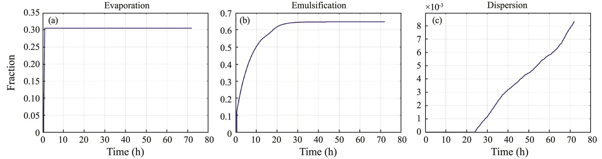
Fig.11 Oil fate processes of the Sanchi oil spill on January 15. (a), evaporation; (b), emulsification; and (c), dispersion.

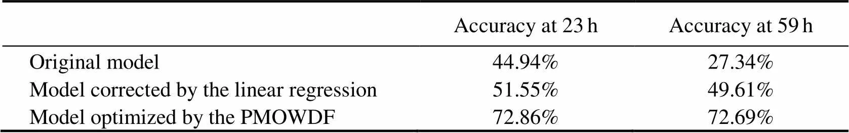
Table 6 Percentage of overlap between the predicted and observed slicks

6 Conclusions

Large amounts of crude oil are frequently spilled dur-ing the exploitation and transportation of oil, resulting insevere marine environmental pollution. Forecasting oil spill trajectories is critical for conducting preventive and effec- tive emergency measures. This paper proposes the PMO-WDF based on deep learning, utilizing the datasets thatcouple the drifter data with the high-resolution wind andcurrent data in 2010–2014. Compared with the empirical parameters in the traditional oil spill model, the method ex-tracts the time-varying features on a regional scale fromthe training data to reduce the random influence of the windparameter in the oil spill prediction. Moreover, the method is adopted into the Eulerian-Lagrangian equation to estab- lish an accurate oil spill prediction model in the East Chi- na Sea. The oil spill trajectories in 2015 with the range of the East China Sea are simulated and validated with drif- ter data, introducing MAE and RMSE as evaluation factors.The Sanchi oil spill that occurred in 2018 is also simulated,setting the overlap ratio between the predicted slick and the satellite observed oil slick as the validation criteria.

The comparison analysis of the PMOWDF and the tra- ditional method revealed that the oil spill forecasts are ef- fectively simulated using the PMOWDF. In the simulation of predicting drifters, the accuracy improvement rate of the PMOWDF compared with the traditional method can range from approximately 5.81% to 11.06%. Meanwhile, the afore-mentioned rate can reach 45.35% and 27.92% at 23 and 59h, respectively, in the Sanchi oil spill simulation. Overall, the study reveals that the wind drift factor is sensitive in oil spill modeling, varying with climatic conditions rather thanremaining constant. Furthermore, employing deep learningto parameterize the wind drift factor can increase the accu- racy of oil spill modeling, which can further improve the ef-ficiency of oil spill recovery and lessen the impact of oil spill disasters.

Acknowledgements

We would like to thank HYCOM for the access to cur- rent datasets from HYCOM (www.hycom.org), wind data-sets from ECMWF (www.ecmwf.int/en/forecasts/datasets), and the drifter data from NOAA’s Atlantic Oceanographic and Meteorological Laboratory (www.aoml.noaa.gov). This research was funded by the Social Science Foundation of Shandong (No. 20CXWJ08).

Abascal, A. J., Castanedo, S., Mendez, F. J., Medina, R., and Lo- sada, I. J., 2009. Calibration of a Lagrangian transport model using drifting buoys deployed during the prestige oil spill., 25 (1): 80-90, DOI: 10.2112/07- 0849.1.

Arbic, B. K., Wallcraft, A. J., and Metzger, E. J., 2010. Concur- rent simulation of the eddying general circulation and tides in a global ocean model., 32 (3-4): 175-187, DOI: 10.1016/j.ocemod.2010.01.007.

Cummings, J. A., and Smedstad, O. M., 2013. Variational data assimilation for the global ocean. In:,. Park, S. K., and Xu, L., eds., Springer-Verlag, Berlin, Heidelberg, 303-343.

De Dominicis, M., Bruciaferri, D., Gerin, R., Pinardi, N., Pou- lain, P. M., Garreau, P.,., 2016. A multi-model assessment of the impact of currents, waves and wind in modelling sur- face drifters and oil spill.–, 133 (SI): 21-38, DOI: 10.1016/j.dsr2. 2016.04.002.

De Dominicis, M., Pinardi, N., Zodiatis, G., and Lardner, R., 2013. MEDSLIK-II, a Lagrangian marine surface oil spill model for short-term forecasting–Part 1: Theory., 6 (6): 1851-1869, DOI: 10.5194/gmd-6-1851-2013.

Elipot, S., Lumpkin, R., Perez, R. C., Lilly, J. M., Early, J. J., andSykulski, A. M., 2016. A global surface drifter data set at hour- ly resolution., 121 (5):2937-2966, DOI: 10.1002/2016JC011716.

Gautama, B. G., Longepe, N., Fablet, R., and Mercier, G., 2016. Assimilative 2-D Lagrangian transport model for the estima- tion of oil leakage parameters from SAR images: Application to the Montara oil spill., 9 (11SI): 4962-4969, DOI: 10.1109/JSTARS.2016.2606110.

Guo, J., Xie, Q., and Liu, X., 2012. Observation of the Penglai 19-3 oil leak and its impact on the sea area ecosystem.. Munich, 919-922.

Guo, W. J., and Wang, Y. X., 2009. A numerical oil spill model based on a hybrid method., 58 (5): 726-734, DOI: 10.1016/j.marpolbul.2008.12.015.

Guo, W., Jiang, M., Li, X., and Ren, B., 2018. Using a genetic algorithm to improve oil spill prediction., 135: 386-396, DOI: 10.1016/j.marpolbul.2018.07.026.

Hodges, B. R., Orfila, A., Sayol, J. M., and Hou, X., 2015. Op- erational oil spill modelling: From science to engineering ap- plications in the presence of uncertainty. In:. Ehrhardt, M., ed., Springer International, Switzerland, 99-126.

Kabdasli, M. S., Kacmaz, S. E., Bas, B., Oguz, E., and Bagci, T., 2010. An oil spill distribution study in an industrial coastal zone., 19 (9A): 1935-1945.

Kampouris, K., Vervatis, V., Karagiorgos, J., and Sofianos, S., 2021. Oil spill model uncertainty quantification using an at- mospheric ensemble., 17 (4): 919-934, DOI: 10. 5194/os-17-919-2021.

Keramea, P., Spanoudaki, K., Zodiatis, G., Gikas, G., and Sylaios,G., 2021. Oil spill modeling: A critical review on current trends, perspectives, and challenges., 9 (2): 181, DOI: 10.3390/jmse9020181.

Khade, V., Kurian, J., Changa, P., Szunyogh, I., Thyng, K., and Montuoro, R., 2017. Oceanic ensemble forecasting in the Gulf of Mexico: An application to the case of the deep water hori- zon oil spill., 113: 171-184, DOI: 10.1016/j. ocemod.2017.04.004.

Khirirat, S., Feyzmahdavian, H. R., and Johansson, M., 2017. Mini- batch gradient descent: Faster convergence under data sparsity.. Melbourne, VIC, 2880-2887.

Kim, T., Yang, C., Oh, J., and Ouchi, K., 2014. Analysis of the contribution of wind drift factor to oil slick movement under strong tidal condition: Hebei Spirit oil spill case., 9 (1): e87393, DOI: 10.1371/journal.pone.0087393.

Lardner, R., and Zodiatis, G., 2017. Modelling oil plumes from subsurface spills., 124 (1): 94-101, DOI: 10.1016/j.marpolbul.2017.07.018.

Leech, M. V., Tyler, A., and Wiltshire, M., 1993. OSIS: A PC- based oil spill information system., 1993 (1): 863-864, DOI: 10.7901/2169- 3358-1993-1-863.

Lehr, W. J., and Simecek-Beatty, D., 2000. The relation of Lang- muir circulation processes to the standard oil spill spreading, dispersion, and transport algorithms.6 (3-4): 247-253, DOI: 10.1016/S1353-2561(01) 00043-3.

Li, M. C., Zhang, G. Y., Si, Q., Liang, S. X., and Sun, Z. C., 2013. Numerical modeling of oil spill with tidal and wind-drivencoupled model in Bohai Bay.,423: 1394-1397, DOI:10.4028/www.scientific.net/AMM.423- 426.1394.

Li, Y., Yu, H., Wang, Z., Li, Y., Pan, Q., Meng, S.,., 2019. The forecasting and analysis of oil spill drift trajectory during the Sanchi collision accident, East China Sea., 187 (106231), DOI: 10.1016/j.oceaneng.2019.106231.

Onay, M. G., Pehlivanoglu-Mantas, E., and Martins, F., 2020. Oil spill modeling in East Mediterranean., 35 (4): 1737-1750, DOI: 10.17341/gazimmfd.534139.

Pan, Q., Yu, H., Daling, P. S., Zhang, Y., Reed, M., Wang, Z.,., 2020. Fate and behavior of Sanchi oil spill transported by the Kuroshio during January-February 2018., 152 (110917), DOI: 10.1016/j.marpolbul.2020.110917.

Pan, Q., Zhu, X., Wan, L., Li, Y., Kuang, X., Liu, J.,., 2021. Operational forecasting for Sanchi oil spill., 108 (102548), DOI: 10.1016/j.apor.2021.102548.

Reed, M., Aamo, O. M., and Daling, P. S., 1995. Quantitative- analysis of alternate oil-spill response strategies using OSCAR., 2 (1): 67-74, DOI: 10. 1016/1353-2561(95)00020-5.

Spaulding, M. L., 2017. State of the art review and future direc- tions in oil spill modeling., 115 (1-2): 7-19, DOI: 10.1016/j.marpolbul.2017.01.001.

Spaulding, M. L., Kolluru, V. S., Anderson, E., and Howlett, E., 1994. Application of 3-Dimensional oil-spill model (WOSM/ OILMAP) to hindcast the Braer spill., 1 (1): 23-35, DOI: 10.1016/1353-2561(94)90005- 1.

Takahashi, D., and Morimoto, A., 2013. Mean field and annual va- riation of surface flow in the East China Sea as revealed by com- bining satellite altimeter and drifter data., 111: 125-139, DOI: 10.1016/j.pocean.2013.01.007.

Timko, P. G., Arbic, B. K., Hyderd, P., Richman, J. G., Zamudio, L., O’Dea, E.,., 2019. Assessment of shelf sea tides and tidal mixing fronts in a global ocean model.. 136: 66-84, DOI: 10.1016/j.ocemod.2019.02.008.

Xu, L., Yang, H., and Wang, C., 2020. Study on oil spill risk as- sessment of oil production platforms in the East China Sea., 39 (2): 260-267 (in Chinese with English abstract).

Yang, H., Han, Z., Li, Y., Wu, Y., and Tang, L., 2012. Numerical simulation of oil-spill in the Xihu Trough of the East China Sea., 31 (2): 216-220 (in Chi- nese with English abstract).

Yang, Z., Shao, W., Hu, Y., Ji, Q., Li, H., and Zhou, W., 2021. Re- visit of a case study of spilled oil slicks caused by the Sanchi accident (2018) in the East China Sea., 9 (3): 279, DOI: 10.3390/jmse9030279.

Yu, F., Fan, Z., Hu, H., Zhao, Y., Tang, J., and Chen, G., 2020. A regional parameterisation method for oil spill susceptibility assessment in Beibu Gulf., 215 (107776), DOI: 10.1016/j.oceaneng.2020.107776.

Yu, F., Xue, S., Zhao, Y., and Chen, G., 2018. Risk assessment of oil spills in the Chinese Bohai Sea for prevention and readiness., 135: 915-922, DOI: 10.1016/j.mar polbul.2018.07.029.

Yu, F., Yao, F., Zhao, Y., Wang, G., and Chen, G., 2016. i4Oilspill, an operational marine oil spill forecasting model for Bohai Sea., 15 (5): 799-808, DOI: 10.1007/s11802-016-3025-6.

Zelenke, B. B., O’Connor, C. C., Barker, C. H., Beegle-Krause, C. J., and Eclipse, L., 2012. General NOAA operational modeling environment (GNOME) technical documentation, data formats. NOAA technical memorandum, NOS-OR&R 41.

Zhang, Y., Yang, T., Zhang, J., Lv, B., Cheng, X., and Fang, Y., 2020. Laboratory investigation into the evaporation of natural- gas condensate oils: Hints for the Sanchi oil spill., 19 (3): 633-642, DOI: 10.1007/ s11802-020-4113-1.

Zhu, K., Mu, L., and Xia, X., 2021. An ensemble trajectory pre- diction model for maritime search and rescue and oil spill basedon sub-grid velocity model., 236: 109513, DOI: 10.1016/j.oceaneng.2021.109513.

Zodiatis, G., Lardner, R., Alves, T. M., Krestenitis, Y., Perivolio- tis, L., Sofianos, S.,., 2017. Oil spill forecasting (prediction)., 75 (6): 923-953.

(March 11, 2022;

June 6, 2023;

August 30, 2023)

© Ocean University of China, Science Press and Springer-Verlag GmbH Germany 2023

. Tel: 0086-532-66782155

E-mail: zhaoyang@ouc.edu.cn

(Edited by Xie Jun)