Specht Triangle Approximation of Large Bending Isometries
2023-12-10XiangLiandPingbingMing
Xiang Li and Pingbing Ming,*
1 LSEC,Institute of Computational Mathematics and Scientific/Engineering Computing, AMSS, Chinese Academy of Sciences, No. 55, East Road Zhong-Guan-Cun, Beijing 100190, China
2 School of Mathematical Sciences, University of Chinese Academy of Sciences, Beijing 100049, China
Abstract.We propose a Specht triangle discretization for a geometrically nonlinear Kirchhoffplate model with large bending isometry.A combination of an adaptive time-stepping gradient flow and a Newton’s method is employed to solve the ensuing nonlinear minimization problem.Γ-convergence of the Specht triangle discretization and the unconditional stability of the gradient flow algorithm are proved.We present several numerical examples to demonstrate that our approach significantly enhances both the computational efficiency and accuracy.
Key words: Specht triangle,plate bending,isometry constraint,adaptive time-stepping gradient flow.
1 Introduction
The geometrically nonlinear Kirchhoffplate models have drawn great attention recently because they capture the critical feature of large bending deformations of thin plates in modern nanotechnological applications [9,19,21,26,29].The dimensional reduced nonlinear plate model has been proposed by Kirchhoffin 1850 [20],which is based on a curvature functional subject to a pointwise isometry constraint.Friesecke and Müller[17]have derived this model from three dimensional hyperelasticity via Γ-convergence.Since then,extensive studies have been carried out from the perspective of modeling and numerics,such as the single layer problem [4,13],the bilayer problem [1,8,12],the thermally actuated bilayer problem [7],just to mention a few.The above models all involve minimizing an energy functional with the isometry constraint.One of the numerical difficulties is the non-convexity of the energy functional caused by the isometry constraint [6].
In this work we focus on the single layer model,and find a deformationy:Ω→R3of a bounded Lipschitz domain Ω⊂R2by minimizing
subject to the isometry constraint
and Dirichlet boundary condition
whereH ∈L2(Ω;R2×2) is the second fundamental form of the parametrized surface given by
and Id2is the identity matrix of order 2.ΓDis part of the boundary ofD.We assume that
The numerical approximation of this problem consists of two parts: discretization and minimization.A proper finite element discretization needs to take into account both high order differential operator of (1.1) and the pointwise isometry constraint.In [4,8],the authors employed a discrete Kirchhofftriangle (DKT),which has been developed in [10] for the linear bending problem.DKT element possess the degrees of freedom of gradient at the nodes,which is convenient for imposing the constraint (1.2).The implementation of DKT element is based on the construction of a discrete gradient operator that maps the gradient to another space.Although this operator makes the proof of Γ-convergence of the discrete energy easier,while its numerical realization is rather complicate.Moreover,DKT is not included in the standard finite element library[13].In addition,the quadrilateral DKT element is not suitable for the adaptive grid refinement.A discontinuous Galerkin (DG) method has been employed in [12,13] to simulate (1.1) and (1.2).DG method has been included in many existing softwares and are more flexible in imposing the boundary conditions,while it needs a careful reconstruction of the discrete energy as well as a fine-tuned penalty factor.
In the present work,we turn to the nonconforming finite element method,in particular we shall exploit the Specht triangle,which is an excellent nonconforming plate bending element [30],and passes all the patch tests and performs excellently,and is one of the best thin plate triangles with 9 degrees of freedom that currently available [33,Quotation from p.345].The Specht triangle has been systematically studied by Shi and his collaborators in [23,27,28,31].Recently the second order Specht triangle has been designed and test in[22].The constraint(1.2)may also be imposed on the nodes,and we prove Γ-convergence ofEhtoEinH1(Ω;R3),which shows the correctness of the energy discretization.
To ensure the energy (1.1) decreases while maintaining the constraint (1.2),a discreteH2-gradient flow method has been designed in [4,6,8,12,13] for geometrically nonlinear Kirchhofftype models.For the single layer plate,the gradient flow exhibits two attractive properties.One is the unconditional energy stability,and the other is that theL1error of the constraint (1.2) is controlled by a pseudo-time step,which is independent of the number of the iteration.However,due to the first-order nature of the gradient flow method,it usually takes a large number of iteration to lower the error committed by the constraint to a reasonable threshold.To speed up the iteration,we shall exploit an adaptive time-stepping strategy developed in [15,24,32] for the phase field models.Compared to [4],our method is around five times faster without loss of accuracy.We combine theH2-gradient flow and a Newton’s method to construct a global-local algorithm that improves the accuracy by around 1~2 order of magnitude and results into a second order method for examples with smooth minimizers.Similar idea has been used in [3] for simulation of the harmonic maps into sphere.
The remaining part of the paper is organized as follows.In Section 2,we use the Specht triangle to discretize the variational problem.The Γ-convergence of the discrete energy to the exact energy is proved in Section 3.In Section 4,we introduce a new method that combines a discrete adaptive time-steppingH2-gradient flow and the Newton’s method.We present numerical experiments and test the accuracy and efficiency of the method in the last section.
2 The specht triangle discretization
We fix some notations firstly.The standard notations for the Sobolev spaces,the norms and semi-norms [2] will be used.The function spaceL2(Ω) consists of functions that are square integrable over Ω,which is equipped with the inner product(·,·)and the norm‖·‖L2(Ω),respectively.LetHm(Ω)be the Sobolev space of square integrable functions whose weak derivatives up to ordermare also square integrable with the norm defined by
where the semi-norm
whereα=(α1,α2) is a multi-index whose componentsαiare nonnegative integers,
Fork ≥0,(Ω) is the closure inHk(Ω) of the space ofC∞(Ω) functions with compact supports in Ω.
For mesΓD0,the following Friedrichs inequality holds: for anyv∈H1(Ω) that vanishes over ΓD,there existsCFdepending only on ΓDand Ω such that
The values of Friedrichs’ constantCFmay be found in [25] for simple domains such as balls,rectangles,etc.
Under the constraint (1.2),the following identity holds pointwise:
which was proved in [12,13].Hence,the energy functionalE[z] may be rewritten into
We reshape the variational problem into
where the admissible set A is defined by
2.1 The Specht triangle
LetThbe a triangulation of Ω with maximum diameterh,and we assume that all the elements are shape regular in the sense of Ciarlet-Raviart [16].We also assume thatThsatisfies the inverse assumption: there holdsh/hK ≤νforK ∈Thand someν >0,wherehKis the diameter of the elementK.We denote the set of all vertices ofThbyVh,the set of all edges ofThbyEh,and the set of all internal edges ofThby.Let∇hbe a piecewise differential operator defined for anyK ∈Thas(∇hz)|K=(∇z)|K.
The Specht triangle is defined by a finite element triple (K,PK,ΣK) as:
whereKis a triangle,andZKis the Zienkiewicz space [11] defined by
and the element bubble functionbK:=λ1λ2λ3withthe barycentric coordinates ofK.
Define the finite element space Xhof the Specht triangle as
The interpolate operate Π associated with Xhis defined locally as Π|K=ΠKfor anyv∈H3(K) and
For allv∈H3(Ω),there holds [16]:
For allk=1,2,3 andv ∈Xh,it follows from the inverse assumption that there existsCinvdepending onνandkbut independent ofvsuch that
2.2 Discrete energy
We approximate(2.2)by the Specht triangle.The function in Xhis continuous over the whole domain and its gradient is continuous at all nodes,which allows us to impose the isometry constraint (1.2) at each node.Define the discrete admissible set by
The discrete energy minimization problem reads as
is in a piecewise manner.
Proposition 2.1.Minimization problem(2.7)has a solution.
The proof is standard,we omit it.
3 Γ-convergence of the discrete energy
The discrete minimization problem (2.7) is non-convex,the standard finite element error analysis fails.Instead,we prove the Γ-convergence ofEhtoEinH1(Ω;R3),which shows the correctness of our energy discretization.Following a standard Γconvergence procedure in [14],we firstly show the compactness and equi-coercivity for anyz∈Ah,and secondly,we prove the lim-sup and lim-inf inequalities.We start with the equi-coercivity of{Eh}h≥0.
3.1 Equi-coercivity and compactness
Lemma 3.1(Coercivity ofEh).Let the data(f,g,Φ)satisfy(1.3).There exists a positive constant C depending onΩ,ΓD and the triangulation,but independent of h such that for any z ∈Ah,
Compared to the known equi-coercivity results in the literature,we clarify the upper bound on the data and the discrete energy functional,and the constantsCin (3.1) and (3.2) may also be elucidated from the proof.
Proof.For anyz∈Ah,letIhbe the linear Lagrange interpolation operator,note the fact that
Applying the Friedrich’s inequality (2.1) toIh(z-g) andIh(∇z-Φ),we obtain
Forj=0,1,we use the standard interpolation estimate forIhand the inverse inequality (2.6) to obtain
Using the triangle inequality,the Friedrichs inequality (3.3) and the interpolation estimate (3.4),we obtain
Using (3.4)2withj=1,we obtain
and using (3.4)1withj=1,we obtain
A combination of the above three inequalities gives
whereA=CF+CIh+CFCICinv.
Proceeding along the same line that leads to the above inequality,we obtain
A combination of the above two inequalities leads to
It is clear that
Using Young’s inequality,we get
This immediately implies
which leads to (3.2).
Substituting the above inequality into (3.5) and (3.6),we obtain
This gives (3.1).
This immediately implies
Proposition 3.1(Equi-coercivity).Let the data(f,g,Φ)satisfy(1.3).The sequence{yh}h>0⊂Ah has a uniform energy bound Eh[yh]≤Λ,whereΛis independent of h.Then the sequence {yh}h>0is uniformly bounded in H1(Ω),i.e.,
with C independent of h.
The uniformly boundedness of{yh}in Proposition 3.1 ensures the existence of a subsequence (not relabeled) of{yh}hsuch that
for somey ∈H1(Ω;R3).We want to show that there existsy ∈A⊂H2(Ω;R3) such that
Proposition 3.2(Compactness inH1(Ω)).Let the data(f,g,Φ)satisfy(1.3).If the sequence {yh}h>0⊂Ah has a uniform energy bound Eh[yh]≤Λfor all h>0,whereΛis independent of h,then there exit y ∈A⊂H2(Ω;R3)and a subsequence(not relabeled)of {yh}h such that
Proof.It follows from Lemma 3.1 and Proposition 3.1 that{yh}hand{Ih(∇yh)}hare uniformH1-bounded,hence there exists a weakly converging subsequence of{yh}hsuch that
for somey ∈H1(Ω;R3) andz ∈H1(Ω;R3×2) ash→0.We apply the standard interpolation estimate forIhand the inverse inequality to get
The uniqueness ofL2weak limit implies∇y=z,and hencey∈H2(Ω;R3).
Moreover,it follows from∇yh ⇀∇yand (3.2) that
It remains to prove thatyis an isometry.
Note thatIh(∇yh)=Id2.Invoking the interpolation estimate and the inverse inequality again,we obtain
where we have used Lemma 3.1 in the last step.
The uniqueness of the weak limit implies thatyis an isometry and this completes the proof.
We are ready to prove Γ-convergence ofEhtoEinH1(Ω;R3).Firstly we extend the domain of discrete energy functional toH1(Ω;R3) as follows.
Theorem 3.1(Γ-convergence).Let the data(f,g,Φ)satisfy(1.3).The following two properties hold
1.Lim-inf inequality:For every sequence {yh}h ⊂H1(Ω;R3)converging to y in H1(Ω;R3),we have
2.Lim-sup inequality:For any y ∈H1(Ω;R3),there exits a sequence {yh}h with yh ∈H1(Ω;R3)such that yh →y and
Proof.We firstly prove the lim-inf inequality.Without loss of generality,we assume thatyh∈Ah⊂H1(Ω;R3) andEh[yh]≤Λ,where Λ is a positive constant independent ofh.Otherwise,
and the lim-inf inequality holds.
Proposition 3.2 implies thaty∈A⊂H2(Ω;R3).We shall show
For anyφ∈(Ω;R3×2×2),using integration by parts,we obtain
For any edgee,there holds
by [27].Hence,for any constant vectorCe,we write
Denotee=K1∩K2,K=K1∪K2.Using the rescaled trace inequalities,we get
Therefore,we obtain
Taking the limith→0,we get
i.e.,⇀∇2yweakly inL2(Ω;R3×2×2).
Next we prove the lim-sup inequality.Without loss of generality,we assume thaty ∈A⊂H2(Ω;R3).The fact that smooth isometries is dense among isometries inH2(Ω;R3) [18] allows us to assume thaty ∈H3(Ω;R3).Letyhbe the Specht interpolant ofy,for alla∈Vh,we get
Henceyh∈Ah.Using the interpolation estimate(2.5),we obtainyh→yinH2(Ω;R3),and whence the convergence of the discrete energy,i.e.,
This completes the proof.
Combining Proposition 3.2 and Theorem 3.1,we obtain that the cluster points of the global minimizers ofEhare global minimizers ofE.
Corollary 3.1.Let data(f,g,Φ)satisfies(1.3).Let {yh}h be a sequence of almostglobal minimizers of Eh,i.e.,
where ∈h→0as h→0and C is a constant independent of h.Then{yh}h is uniformly bounded in the H1norm,and every cluster point y of {yh} is a global minimizer of E,i.e.,
Moreover,there exits a subsequence of {yh}h(not relabeled)such that
4 A combination of the gradient flow and Newton’s method
TheH2-gradient flow algorithm developed in [4] is an efficient method to solve the problem with constraints,while the first oder convergence rate seems a hurdle for efficient implementation.To speed up the iteration,we firstly adopt theH2-gradient flow method with an adaptive time-stepping technique,which is based on the energy variation;Such techniques appeared in the simulation of the phase field model in[24];See also [15,32].Secondly,we combine the gradient flow and a Newton’s method.
4.1 H2-gradient flow
At a pointyh∈we define the tangent space Fh[yh]of the admissible space Ahby
Letτ >0 be a pseudo-time parameter,∈Ahbe the initial deformation,and∈be the stopping threshold.Define
At (k+1)-th step,we solve
where we have included a regularized term
to ensure the energy decay.Until the stopping criterion
Theorem 4.1.Letbe the k+1-th step solution of the gradient flow(4.2),thereholds
1.Energy decay:
2.Isometry violation:
Proof.Choosingv=in (4.2),and using the elementary identity
which implies
Using the telescoping sum,we obtain (4.3).
Note that for alla∈Vh,there holds
By the definition ofin (4.2),we get
On every nodea∈Vh,we have
Leta,b,cbe the three vertices of the elementK,a direct calculation gives
Invoking the Friedrichs inequality (2.1) and the energy decay estimate (4.3),we obtain
This completes the proof.
4.2 Adaptive time-stepping method
The simulation of the large bending problem needs long time computations,and the adaptive time-stepping method seems a natural choice.Theorem 4.1 implies that theH2-gradient flow method is unconditionally stable,and the accumulation of isometry violation is related to the energy drop at each step.Therefore,we adopt a time step adaptive approach based on the energy variation to accelerate the iterations while maintaining the accuracy.Such time step adaptive strategy has been developed in [15,24,32] for the phase field models.The choice of the step sizeτk+1is based on the variations of the energy
during the gradient flow iteration.In particular,if the energy changes smoothly,then the step size will be increased to accelerate the convergence.On the other hand,if the energy is changing rapidly,the step size will be decreased to maintain the isometry constraint.
At (k+1)-th step,we adjust the time stepτk+1as
where the parametersτmaxandτminrepresent the maximum and minimum step lengths,respectively,andαis a case dependent parameter.
4.3 Newton’s method
Unlike the gradient flow method,which has global convergence properties,the Newton’s method is a local method,which achieves a second order rate of convergence once a good initial point is chosen.Thus we apply Newton’s method with the starting point obtained by the gradient flow method.Moreover,we find numerically that Newton’s method efficiently reduces the violation error of the isometry constraint.
Three constraints of isometry [∇yh](a)=Id2on every nodea∈Vhare
We write the discrete Lagrangian as
5 Numerical experiments
We list the basis functions of the Specht triangle[27]for the sake of implementation.Fori=1,2,3,
whereζi,θi,ωiare basis functions associated with the degrees of freedomv(ai),∂xv(ai),∂yv(ai),respectively.
Define
to measure the violation of the isometry constraint.It follows from Theorem 4.1 thatI1h[yh] is ofO(τ).Similarly,we define
as another measurement for the violation of the isometry constraint.It follows from the estimate (3.7) thatI2h[yh] is bounded byO(h).Finally,we defineKh[yh] as theL1error of the discrete Gaussian curvature ofyhas
wherenh=∂1yh×∂2yhdenotes the outer normal vector of the solution surface.Under isometry constraint,Gauss theorem egregium implies that Guass curvature of every point of the exact solution should vanish.
The linear system of thek-th step gradient flow iteration is
whereSis the stiffmatrix andBkencodes the linearized isometry constraint.
The linear system of thek-th step of Newton’s method is
where the two extra itemsFλandSλcome from the exact isometry constraint in Lagrangian multiplier terms ofL(yh,λh).We note that the cost of each iteration of Newton’s method is similar to that of the gradient flow.
Our numerical examples are motivated by [4] and [13].We chooseτmin=h,τmax=10h,α=1e5 and∈=1e-3 unless otherwise stated.We firstly consider a simple example to test the numerical performance of our method for a relatively smooth deformation.
Example 5.1(Rectangular plate under vertical load).Let Ω=(0,4)×(0,1).We consider the clamped boundary condition
on part of the boundary ΓD={0}×[0,1],and we apply a constant vertical forcef(x)=(0,0,2.5×10-2)⊤on the whole domain Ω.
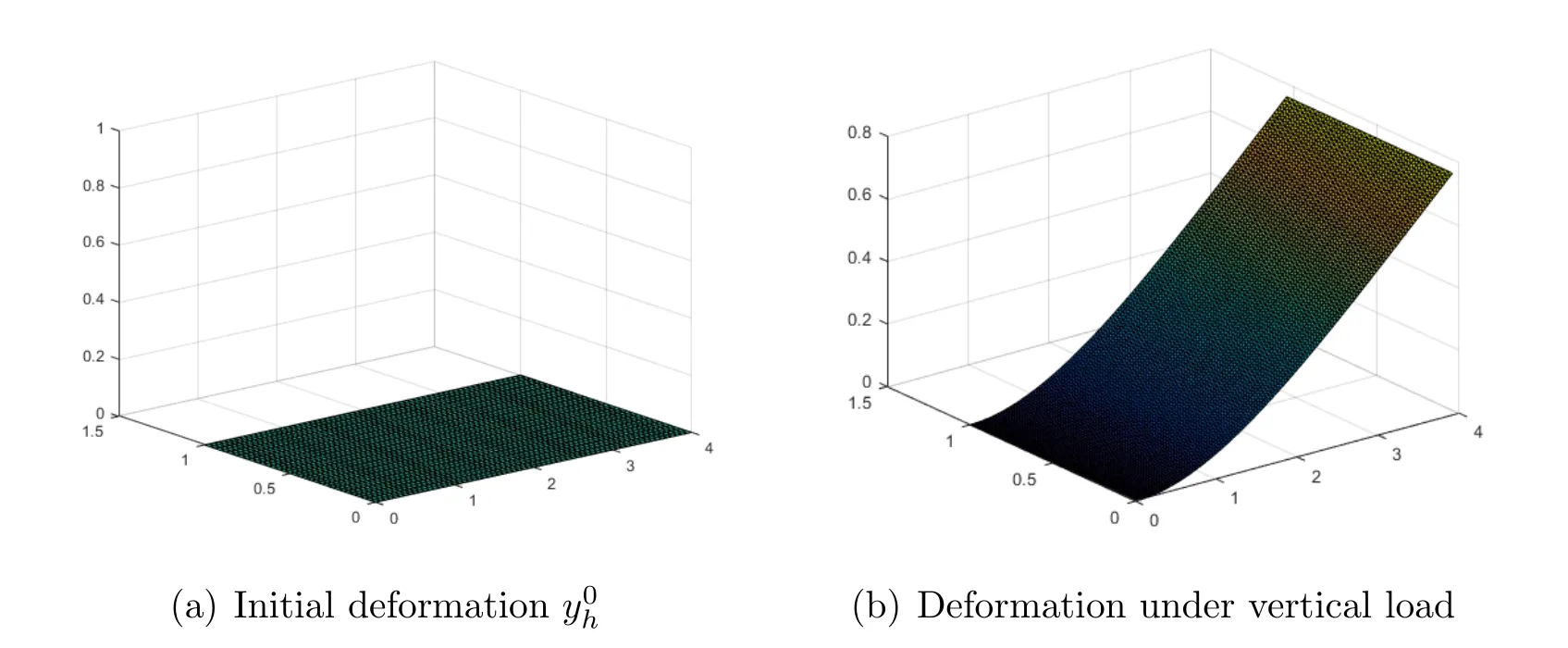
Figure 1: The plate is clamped on one side and the vertical load is applied on the opposite side.
In view of Table 1,we apply the gradient flow iteration on a sequence of triangulationT2,T3,T4andT5,and takeτmin=h,τmax=10h.The energy of the final configuration is-1.58e-2,while the convergence rate of bothI1handI2hare around 1,which is consistent with Theorem 4.1.In view of Table 5,a significantimprovement inI1handI2hhas been observed with two extra Newton’s iterations.Compared to [5],the error ofI2his 1~2 order of magnitude smaller,while only one sixth number of the iteration steps have been used.In view of Table 3,I2hconverges with second order,which is better than the first order rate observed in[4]and superlinear convergence observed in [13].

Table 1: The Specht triangle and H2-gradient flow (τmin=h).
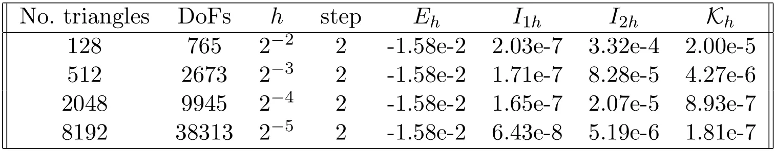
Table 2: Newton’s method (τ=h) with ykh from Table 1 as an initial guess.
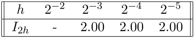
Table 3: Convergence rate: a combination of the gradient flow and the Newton’s method.
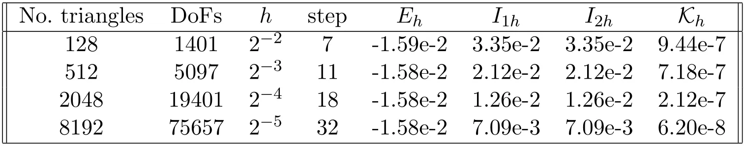
Table 4: The quadratic Specht triangle and H2-gradient flow (τmin=h).
Table 5: The quadratic Specht triangle discretization with Newton’s method: τ=h and from Table 4 has been used as the initial guess.
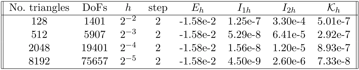
Table 5: The quadratic Specht triangle discretization with Newton’s method: τ=h and from Table 4 has been used as the initial guess.
In what follows,we test the same example with the quadratic Specht triangle developed in [22] with the parametersα1=18 andα2=α3=-45 as the spatial discretization††There are many choices of the quadratic Specht triangle,we take the one with the best numerical performance in [22]..It follows from Table 4 and Table 1 that the method with the secondorder Specht triangle yields almost the same values forI1handI2h.Nevertheless,it is clear in Table 4 that the accuracy is improved to certain degree forI1h,I2handKhif we combine the Newton’s method with theH2-gradient flow method.
Example 5.2(Square plate under vertical load).Let Ω=(0,4)×(0,4).We consider the clamped boundary condition
on part of the boundary ΓD={0}×[0,4]∪[0,4]×{0},and we apply a constant vertical forcef(x)=(0,0,2.5×10-2)⊤on the whole domain Ω.
In view of Table 6,we apply theH2-gradient flow algorithm with adaptive timestepping to a sequence of triangulationsT2,T3,T4andT5.The convergence rates of bothI1handI2hare still around 1,and the number of the iteration steps of our method are robust to the variation of the mesh size.
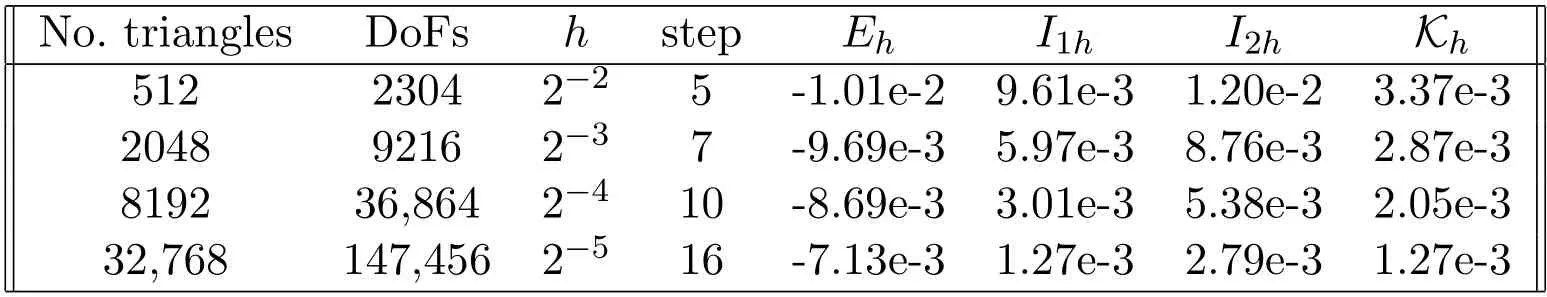
Table 6: The Specht triangle and H2-gradient flow.

Figure 2: vertical load.
In view of Table 7,compared to [4] and [13],our adaptive strategy significantlyreduces the number of the iterations.In particular on the triangulationT5,the DKT element in [4] requires 130 iteration steps,and the DG method in [13] requires 140 iteration steps,while our method achieves the same accuracy as [4] with only 16 iteration steps.

Table 7: Comparison of DKT [4],DG method [13] and our method (without Newton’s method) of the same example on the triangulation T5.
In view of Table 8 and Table 9,Newton’s method is effective in reducingI1h.However,I2hremains at a similar magnitude and the convergence rate is only around 1.This could be attributed to the way the isometry constraints (1.2) is imposed,as well as the nature of the example,which is highly prone to the violation of the isometry constraint.
Table 8: Newton method with from Table 6 as the initial guess.

Table 8: Newton method with from Table 6 as the initial guess.
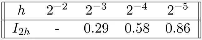
Table 9: Convergence rate: a combination of the gradient flows and Newton’s method.
Another attractive example is the bulking of a plate.
Example 5.3(Buckling: compress a strip).Let Ω=(-2,2)×(0,1).We impose the compressive boundary conditions
on the two sides ΓD={-2,2}×[0,1],and we apply a constant vertical forcef(x)=(0,0,1.0×10-5)⊤over the whole domain Ω.
We choose the initial deformationas
We plot the initial guess and the deformed state in Fig.3.
Note that the initial guess is incompatible in the sense that

Figure 3: Buckling.
which yields a relatively high initial energywe hence adjust the parameters of the adaptive time-stepping toτmax=100τminandα=1e4.
By Fig.3,a bulking deformation occurs,and we display the results in Table 10,and it seems challenging to maintainI1handI2hin this example.
In Table 11,we fix the mesh size ash=2-5and takeτminto beh1/2,h,h3/2,respectively.It takes 367 steps to reduceI2hto 9.82e-2,whereas the author in [4]required 2,457 steps to reduceI2hto 6.91e-2 withτ=h3/2.

Table 11: H2-gradient flow: h=2-5,pseudo-time step,the number of the iteration step, L1-norm of the violation of the isometry,energy.
Next we use resultsykhfrom Table 10 as an initial guess of Newton’s method,and still take∈stop <1e-3.Table 12 shows thatI1hmay be reduced to 1e-8,andI2hmay be reduced to 1e-3 after several additional Newton’s iteration steps.
Table 12: The Specht triangle and the Newton’s method with from Table 10 as an initial guess.
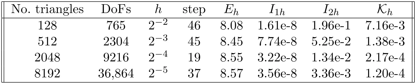
Table 12: The Specht triangle and the Newton’s method with from Table 10 as an initial guess.
Acknowledgements
This work is supported by National Natural Science Foundation of China through Grants No.11971467 and No.12371438.
杂志排行

Annals of Applied Mathematics的其它文章
- Preface
- A Discontinuity and Cusp Capturing PINN for Stokes Interface Problems with Discontinuous Viscosity and Singular Forces
- Connections between Operator-Splitting Methods and Deep Neural Networks with Applications in Image Segmentation
- Fast High Order and Energy Dissipative Schemes with Variable Time Steps for Time-Fractional Molecular Beam Epitaxial Growth Model
- A Review of Process Optimization for Additive Manufacturing Based on Machine Learning
- The Acoustic Scattering of a Layered Elastic Shell Medium