Fast adaptive regression-based model predictive control

Eslam Mostafa·Hussein A.Aly·Ahmed Elliethy

Abstract Model predictive control(MPC)is an optimal control method that predicts the future states of the system being controlled and estimates the optimal control inputs that drive the predicted states to the required reference.The computations of the MPC are performed at pre-determined sample instances over a finite time horizon.The number of sample instances and the horizon length determine the performance of the MPC and its computational cost.A long horizon with a large sample count allows the MPC to better estimate the inputs when the states have rapid changes over time,which results in better performance but at the expense of high computational cost.However,this long horizon is not always necessary,especially for slowly-varying states.In this case,a short horizon with less sample count is preferable as the same MPC performance can be obtained but at a fraction of the computational cost.In this paper,we propose an adaptive regression-based MPC that predicts the best minimum horizon length and the sample count from several features extracted from the time-varying changes of the states.The proposed technique builds a synthetic dataset using the system model and utilizes the dataset to train a support vector regressor that performs the prediction.The proposed technique is experimentally compared with several state-of-the-art techniques on both linear and non-linear models.The proposed technique shows a superior reduction in computational time with a reduction of about 35–65%compared with the other techniques without introducing a noticeable loss in performance.

Keywords Regression analysis·MPC·Control·Parametrization·Wavelet·Support vector regression(SVR)·Optimization

1 Introduction

Model predictive control(MPC)[1]is an advanced control method that has been widely used in many applications[2–6].Given a discrete system with its states defined at specific sampling instances,the MPC utilizes the mathematical model of the system to predict its future states at each sample instant over a finite future horizon time.The predicted states along with a set of given system constraints are used to formulate an optimization problem that is solvedonlinein every control cycle to estimate the optimal control inputs at each sample instant over the horizon.Only the estimated input at the first sample instant is applied to the system,and the MPC repeats the same process for all subsequent control cycles.For a long horizon with a large number of sample instances,the predicted behavior of the system becomes more intimate to the required reference[7],i.e.,better control performance.However,for such a long horizon,the MPC easily may not finalize the computations involved in solving the online optimization problem within the control cycle,and this results in a lagging control input to the system in this case.

To avoid the aforementioned lagging control input problem, several studies in the literature focus on speeding up the MPC by reducing its online computations.For example,several techniques try to minimize the number of sample instances within the horizon.In [8–10], the input and state trajectories,that represent their variations over time,is parametrized with some basis functions.The parameterization of the trajectories reduces the degrees of freedom of the online optimization problem by calculating the control inputs only at specific sampling instances in the horizon while evaluating the rest using the parametrized version.In [11–13],non-uniformly spaced sample instances are used such that smaller intervals between sample instances are used with the near future of the horizon while larger ones are used with the distant future.These techniques use a fixed horizon but keep the number of sample instances relatively small.However,using a fixed horizon is not optimal in all control scenarios.As shown in[14],a short horizon is enough for controlling a vehicle on highways where speed fluctuations are not fast,while a longer horizon is needed when driving in a city due to higher fluctuations in speed and environmental variables.Following this,the technique in[15]adaptively changes the horizon according to the curvature value for the state trajectories.However,thetechniqueusesaheuristicruletodetermine the horizon length,which results in a sub-optimal horizon.In[16],a variable horizon MPC is achieved by defining several fixed-horizon optimization problems with different horizon lengths.The overall complexity is relatively reduced by utilizing the time-varying move blocking technique[17]which fixes adjacent in-time decision variables of the optimization problem or its derivatives to be constant over several control cycles,andthus it results insub-optimal control performance.In[18],the horizon length is added as an extra degree of freedom to the MPC formulation, and thus it incurs additional computations in the control cycle.The technique in[19]deals with systems with non-linear dynamics and incrementally adjusts the horizon length to its minimum possible value that guarantees stabilization.This incremental adjusting for the horizon is practically not suitable for fast applications.

Another line of research is the so-called explicit MPC[20–22],which pre-computes the optimal control inputsofflineas a function of the current state and reference states.Thus,the online optimization reduces to a simple search within the precomputed values.The major drawback here is the searching time for the optimal solution which quickly increases when the number of states,horizon length,or the number of control inputs increases.Thus the explicit MPC can only be applied to small problems.This drawback is partially mitigated in[23]which uses a partial enumeration technique that offline computes and stores in a table the optimal control inputs for only frequently occurring constraint sets.The table is searched online for the best control and updated to incorporate new constraint sets as the control progresses in time.

Recently,machine learning techniques are employed for horizon prediction.In[24,25],a novel technique is proposed that uses reinforcement learning(RL)[26]to predict the optimalhorizonlengthusingapolicyfunctionofthecurrentstate.The policy of the RL is modeled as a neural network(NN)[27]which is trained using the data collected during the operation of the system being controlled.The training of the NN is performed online within each control cycle, which adds more computations within the cycle.Another technique in[28] trains a NN offline that is used to predict the optimal horizon at run-time.However,these techniques perform the prediction solely based on theinstantaneousstate of the system, without any consideration for the future values of the states.Moreover,the techniques do not employ any feature engineering for training the NN, and thus it easily over-fits the training data.Additionally,the technique in[24]predicts the horizon length only while the technique in[28]uses the move-blocking strategy[17]that fixes the ratio between the numberofsampleinstancesandthetimespanofthepredicted horizon.Therefore,the predictions performed by these techniques are not optimal in general.

In this paper, our goal is to accurately estimate both the best minimum horizon length and the number of samples without introducing a noticeable loss in the performance of the MPC.To this goal,we first propose a mathematical formulation that relates the horizon length and the sample count with the performance of the MPC,then we propose an efficient solution for it.Specifically, we propose an adaptive regression-based MPC(ARMPC)that predicts the best minimum horizon length and the sample count according to the current and future variations exhibited in the reference states of the model.To train the regression,we build a dataset by extracting several features that capture the variations of the reference trajectories of the model over future time with the associated best horizon and sample count in each situation.In run time, we extract the same set of features which presented to the regressor to predict the best minimum horizon length and the sample count.

Compared with previous techniques, our proposed ARMPC has several advantages.First,it estimatesboththe best horizon length and the best number of samples on the horizon, and this allows the proposed technique to provide more reduction in computations.Second,our technique does not rely on raw values of the reference states but employs feature engineering to extract several distinctive features from the reference trajectories, and thus it avoids over-fitting in the learning phase.Finally, these features are extracted not from the instantaneous values of the states but over a future span of the horizon,which allows a more accurate estimate for the horizon and the sample count.These advantages are reflected in our experimental results where we compared the proposed ARMPC with three different state-of-the-art techniques on both linear and non-linear models.The proposed ARMPC shows a superior reduction in computational time with a reduction of about 35–65% compared with the other techniques without introducing a noticeable loss in performance.The source code of the proposed technique is available1https://github.com/ahmed-elliethy/fast-regression-mpc.online.

The remainder of this paper is organized as follows.Section2 presents a background for the MPC and briefly outlines its parametrization.Section3 presents motivation examples and formulates our problem statement.Section4 introduces the proposed adaptive regression-based MPC.Section5 describes the experimental setup and discusses the experimental results that evaluate our proposed technique.Section6 summarizes our conclusion and presents our future work.

2 MPC background

A continuous linear time-invariant system can be described in state space form as[10]

wheret∈R is a continuous time instant,x(t) ∈Rm×1andu(t) ∈Rn×1represent a vector of states and a vector of system inputs at timet,respectively,A∈Rm×mis the state matrix,andB∈Rm×nis the input matrix.The system can be discretized using any of the discretization methods(such as the Euler method)by

wherek∈Z is a discrete-time instant,tsis the sampling time,andrepresents the vector of states atk.With the discretization,(1)can be written as

The goal of MPC is to estimate the optimal vector of system inputs for a fixed horizon length ofTtime steps in control cycles.More clearly, in thecth control cycle, the MPC estimates the optimal vector of system inputs from the time instantctoc+T-1.Then only the first control input(at the time instantc)is applied to the system and new system states are predicted.In the next cycle,the MPC estimates the system inputs using the newly predicted states,then only the first input is applied again to the system.This loop will be repeated to find the optimum control input in every control cycle.

To do so,in thecth control cycle,the MPC first expresses the system states as a function of only the inputs and the initial statexcin the cycle as

where

where

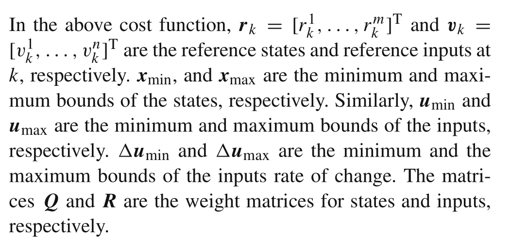
Within the sampling timets, the MPC controller should solve the optimization problem in(4)to find the optimal control inputs and apply the first control input to the system,at every control cycle.However, the solution time of (4) may exceedts, especially for long horizonT, and thus the controller gives a lagging input to the system in this case.In the following, we discuss the idea of parametrization that reduces the computational time of solving(4).

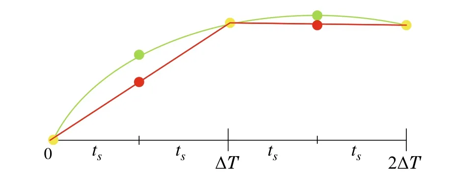
Fig.1 An example of T = 5 control inputs parameterized by P = 3.The green circles represent the instances at which the control inputs are computed without parametrization.After parametrization,the computations are conducted only at the yellow circles,while the other red points are linearly interpolated

2.1 Parametrization

The optimization function in(4)is solved to findTvectors of system inputs.By parametrizing the input trajectories with some basis functions,the optimization(4)is solved but for a fewer number of control inputs.Specifically, the system inputs are estimated only at specific sample instances over the horizonineverycontrolcycle,whiletherestisevaluatedfrom the parameterized version.Without loss of generality, we build our discussion here upon the parametrization technique in [10], which simply linearizes the trajectories with line segments,as shown in Fig.1.

LetPrepresents the number of sample instances over the horizonTat which the control inputs are estimated from the optimization (4) (such as the yellow points in Fig.1).The distance between these sample instances in the unit of time steps can be expressed as

The inputukcan be derived by linear interpolation of the inputs at the next sampleknand the previous onekpas

where

By modifying the dynamic equation(3)byukin(6),we get

thus,the cost function(5)is modified to be

s.t.the same constraints as in (5), whereΥ= {c,c+ΔT,...,c+(P-1)ΔT}.Now,

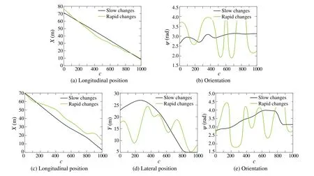
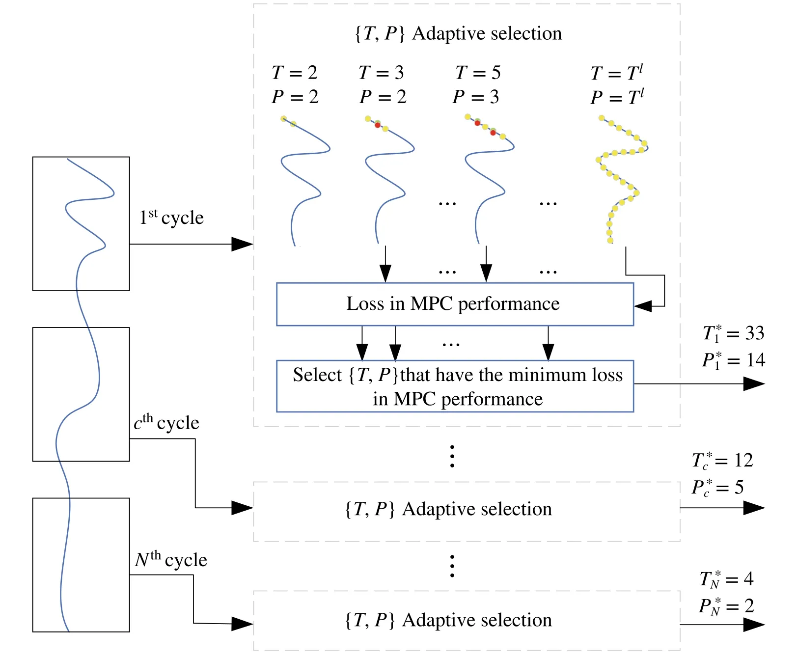
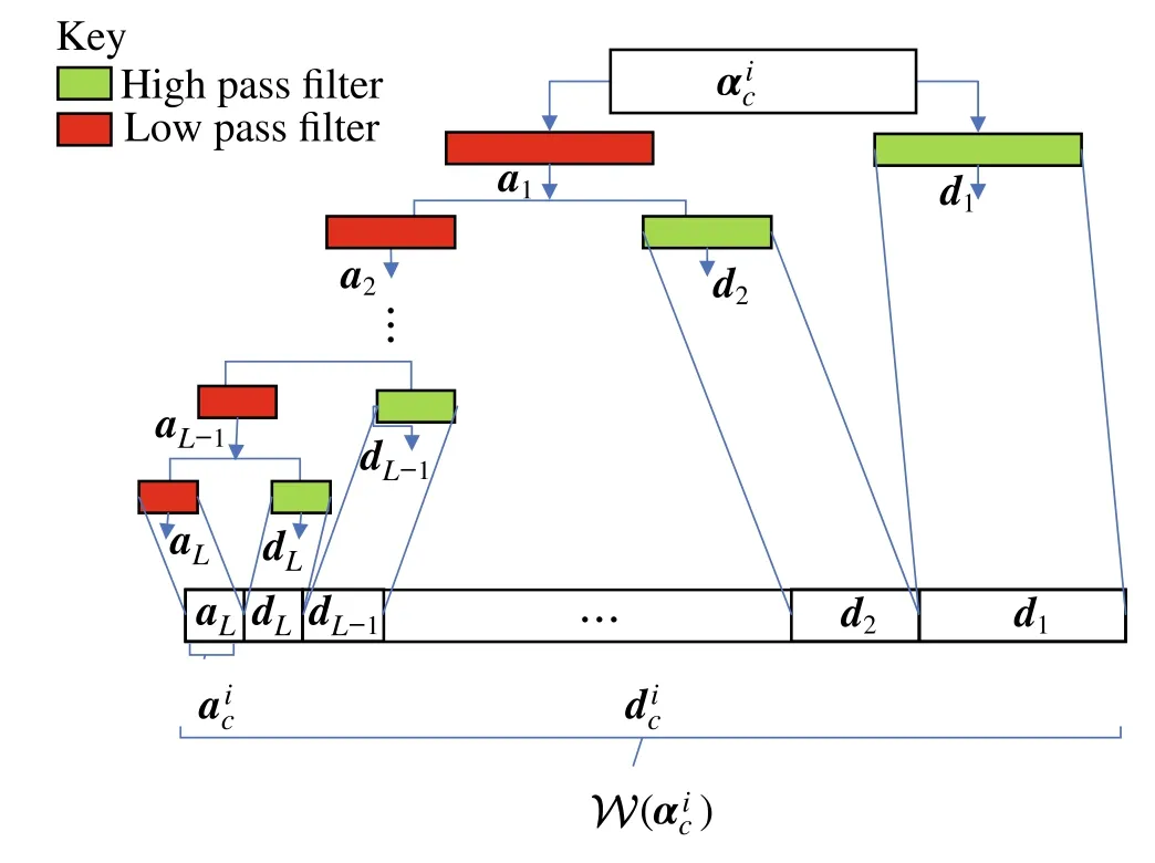
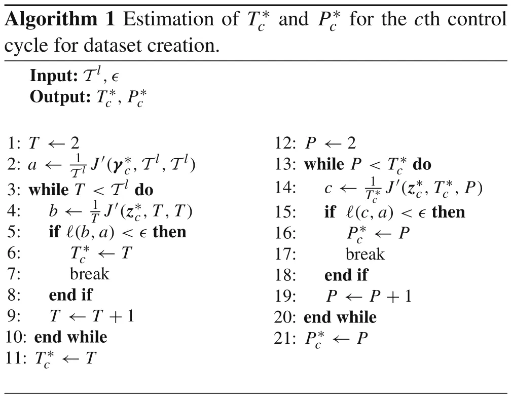
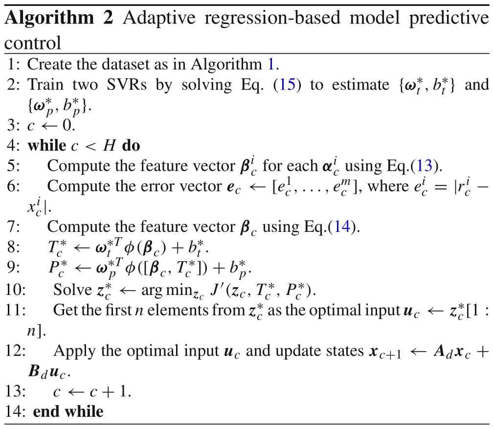
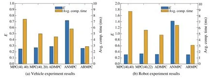
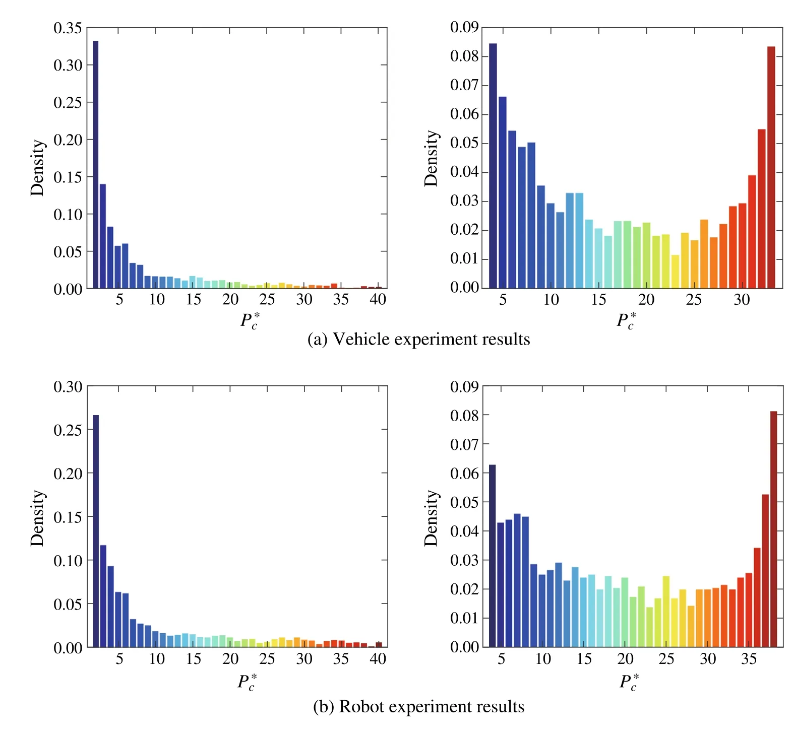
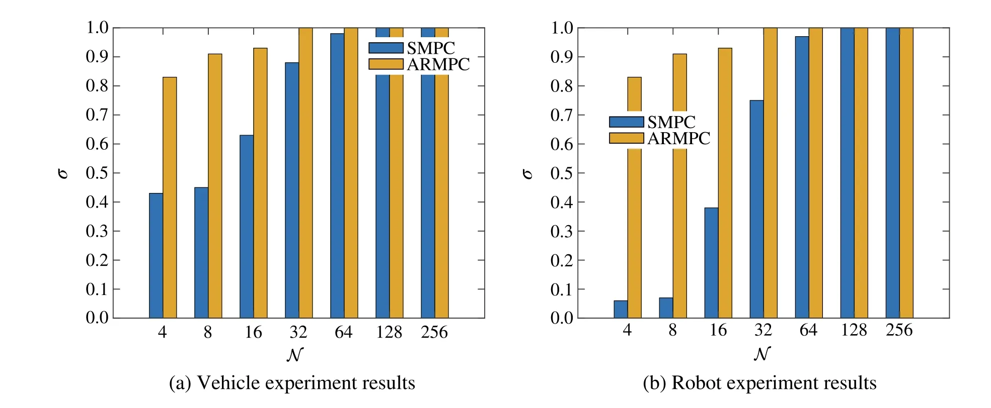
This makes the optimization to be solved onP

3 Motivation and problem statement

As shown in (8), there are two factors that strongly affect both the computational burden and the performance of the MPC,which are the horizon lengthTand the sample countP.To enhance the performance of the MPC,bothTandParefixedto specific large values for all control cycles.When the trajectories of states have rapid changes over future time,the MPC takes the advantage of largeTandPfor better preparing the appropriate inputsz∗c.This allows the MPC to avoid the overshoot that may occur at these rapid changes,which results in better performance but at the expense of more computational cost.However,fixingTandPare not optimal for all trajectories in every control cycle.For example,if the trajectories do not show too many variations,then we can use smaller values forTandPto solve (8) without noticeable loss in control performance but at much less computational cost.This means that it is better to set a variable value forTandPfor every control cycle according to the variations exhibited in the trajectories.In the rest of the paper,we represent thevariablehorizon length and sample count asTcandPc,respectively,for thecth control cycle.In the following, we first present an experimental validation that illustrates the effect of different fixed settings forTandPon both the MPC’s computational time and performance followed by our problem statement that mathematically formulates the problem of adaptive selection ofTcandPcin every control cycle.

3.1 Motivating examples

Fig.2 The vehicle’s state reference trajectories are presented in a,b.The robot’s state reference trajectories are presented in c–e.The black line represents a reference trajectory that is characterized by slow changes,while the green line represents a reference trajectory that is characterized by rapid changes

We validate our claim on two different models.The first model is a linear vehicle model that is built based on a simple bicycle model approximation of a vehicle and we control the vehicle’s lateral position and orientation.The second one is a more complex non-linear robot model that is linearized around the operating point using Linear parameter varying(LPV)[29]which encapsulates the nonlinearity of the robot model into a linear form.We control the position and orientation of the robot.Both vehicle and robot models are presented withmoredetailsinSect.S.IandSect.S.II,respectivelyinthe supplementary material.Figure2 shows the reference state trajectories for both the vehicle and the robot.As shown in the figure, two different sets of reference state trajectories are examined,the first set has slow changes(shown in black color) while the second one has rapid changes (shown in green color).

We run our experiments using four different settings forTandPof the MPC.To differentiate between these settings,we denote MPC(a,b)for a specific setting ofTtoaandPtob.The four settings used in our experiments are MPC(40,40),MPC(5,5),MPC(40,3),and MPC(40,25).Thus,the first two settings are concerned with both long and short values forT,respectively,without parametrization,i.e.,P=T.The other two settings are concerned with a longT,but with different settings forP.We evaluate the performance of the MPC with every setting with both the average computational time and the average cost over all control cycles.Assume that we haveHcontrol cycles,2We used the same H for all experiments.the average costEis computed as

In Fig.3,we plot both the average costEand the average computational time for the four different settings.As shown in the figure,if the reference state trajectories exhibit rapid changes,the average cost becomes very large when using a short horizon or using a long horizon with a small number of sample counts, but the computational time, in this case,is relatively small.For the same trajectories, when using a long horizon or using a long horizon with a sufficient number of sample counts,the average cost becomes smaller but at the expense of more computational time.In the case of reference state trajectories with slow changes, the average cost becomes small, i.e., good performance, for all different settings used in the MPC even with short horizons or a small number of samples.However,this good performance is obtained in a much smaller computational time when using short horizons or a small sample count.

From the results,we can conclude that despite increasing the horizon length and sample count improving the control performance in general,it is not required in all situations.In real scenarios, the state trajectories may exhibit both rapid and slow variations.Therefore, the horizon length and the sample count should not be fixed and should be adaptively selected according to the variations encountered in the state trajectories in every control cycle.With this adaptive selection,the computational cost of the MPC is reduced,while it maintains its performance unaffected.

Fig.3 Plot of the average computational time and the average cost against different settings of MPC for a the vehicle and b the robot.If the reference state trajectories exhibit rapid changes,the average cost is large when using a short horizon MPC(5,5)or using a long horizon with a small sample count of MPC(40,3).For slow variations, the average cost becomes small for all settings.However,the computational time is much smaller for short horizons MPC(5,5)or for a small sample count MPC(40,3)

3.2 Problem statement

A pictorial representation of our problem is shown in Fig.4.According to the situation of the trajectories in thecth control cycle,the values ofTcandPcshould be selected as minimum as possible such that the performance of the MPC is not deteriorated compared with its performance when using large values for horizon length and sample count.LetT lrepresents this large value,then our problem can be formulated as

where∊is a small positive number andγ∗is the vector of optimal control inputs that is estimated when usingT lfor both the horizon length and the sample count.In our formulation,we assess the loss in performance of MPC byℓwhich measures the relative difference of the average of the cost functionJ′(7) when using the values of {T,P} instead ofT lfor both horizon length and the sample count,i.e.,

A possible solution for(10)is that,in every control cycle,we can start with small values ofTandPthen iteratively increment both values until {T∗c,P∗c} are estimated.However,this solution is not practical in run time(i.e.,when the controller is in action)as it involves solving the MPC optimization (8) several times in every control cycle to obtain{T∗c,P∗c}.In the following section,we present our proposed efficient approach to estimate{T∗c,P∗c}.

4 Proposed adaptive regression-based MPC

In this section, we present our adaptive regression-based MPC(ARMPC)scheme which adaptively estimate{T∗c,P∗c}in every control cycle from (10) using a regression model.Our proposed approach is illustrated in Fig.5.Specifically,we build a dataset to train a regression model, then we used the regression model to predict{T∗c,P∗c}.The predicted{T∗c,P∗c}are used to estimate the required control inputsz∗cfrom (8) as usual.In the following, we discuss the feature extraction,the dataset creation,and the regression model in more detail.

Fig.4 Problem statement architecture:In each cth control cycle,we need to determine what is the most suitable{T,P}to be used in MPC optimization

Fig.5 The overall architecture of the proposed regression-based MPC.At each control cycle, reference state trajectories along with the current states of the system being controlled are passed through a feature extractor,then the extracted features are fed to the regression model to predict T∗c and P∗c that will be used by the MPC in this control cycle

4.1 Feature extraction

• CurvatureC()is a value that quantifies the amount by whichdeviates from being a straight line.Mathematically[30],

where

Fig.6 Wavelet decomposition

• Wavelet coefficientsW(αic)which are extracted fromαicusing the wavelet decomposition described in the pyramid architecture in Fig.6.Specifically, two sets of coefficients are computed fromαic: approximation coefficientsaciand detail coefficientsdci[31].The approximation and the detail coefficients are computed by convolvingαicwith a low pass filter and a high pass filter, respectively, followed by dyadic decimation.The same procedure is repeatedLtimes with the approximation coefficients and all resultant coefficients are used to formW(αic).The wavelet decomposition is used in our features because it localizes the trajectory in both time and frequency[31].Thus,a stretched wavelet helps capture the slowly varying changes in the state trajectory while a compressed wavelet helps capture abrupt changes in the state trajectory.

Thus,

Besides capturing the variations in the reference state trajectory, we augment our features by the error vectorec=[e1c,...,emc], whereeic= |ric-xic| represents the absolute error between the values of the reference state and the current state at the time instantc.The reason for taking the error into account is that the error has a noticeable effect on the selection of horizon length and sample count.When the error is large, it is preferred to use large values for both horizon length and sample count to perfectly derive the states to their reference.After we computeβicfrom eachαic, we concatenate the vectorsβicfor alli= 1,...,malong with the error vectorecto form the complete feature vectorβc,i.e.,

To generate the reference states trajectories for feature extraction, we synthetically utilize the discrete state space equation(2)for a given model by randomly varying the control inputs,while satisfying their constraints.

4.2 Dataset creation

We build the dataset by associating each feature vectorβcof thecth control cycle with its corresponding values of the best minimum horizonT∗cand sample countP∗c.Algorithm 1 illustrates how {T∗c,P∗c} are obtained.Specifically,our dataset is built in two successive steps.First,we estimateT∗c, then we estimateP∗cfor the specific estimatedT∗c.To estimateT∗c,we initially set both the horizon length and the sample count to a small valueT,then iteratively incrementTand solve(8)with both horizon length and sample count set toT.In each iteration,the loss in performance(11)of the MPC is computed.If the loss falls below a threshold∊,T∗cis estimated and the iterations are stopped.Otherwise,T∗cis set to the maximum allowable horizon lengthT l.Once we obtainT∗c,we estimateP∗cin the next step.We set the sample count to a small valueP, then iteratively incrementPand solve(8)with horizon length equal toT∗cand sample count set toP.In each iteration,the loss(11)is computed and if it falls below∊,the value ofP∗cis returned.

Algorithm 1 Estimation of T∗c and P∗c for the cth control cycle for dataset creation.Input:T l,∊Output:T∗c ,P∗c 1: T ←2 2: a ← 1 Tl J′(γ∗c,T l,T l)3: while T

Algorithm 1 has high computational cost as it involves solving the MPC optimization (8) several times to obtain{T∗c,P∗c}.However, all these computations are performed offline,i.e.,in the training time.But,once the dataset is built,we predict the values of {T∗c,P∗c} in run time using very simple calculations,thanks to the regression model that we discuss next.

4.3 Regression analysis

Our training dataset containsNrecords, one for each control cycle.Every record is composed of the feature vectorβcfor thecth control cycle with its corresponding values of{T∗c,P∗c}.Our goal here is to build two regression models,the first is for predicting the horizon length and the second one is for predicting the sample count,from the given feature vector.We used the non-linear support vector regression(SVR)[32] technique for building our regression models because of its robustness to outliers,excellent generalization capability,and high prediction accuracy.The objective of the SVR is to find the hyperplaneωTφ(βc)+bthat holds maximum training observation within the marginτ(tolerance level),as shown in Fig.7,whereφ(βc)is a transformation that mapsβcto a higher-dimensional space.Mathematically,the goal of the training of the SVR model is to find the best parametersω∗for the hyperplane by solving

whereC>0 is a regularization parameter that penalizes the number of deviations larger thanτ.Theζ+candζ-care slack variables that allow the regression to have errors,as shown in Fig.7.

We used the same formulation (15) to train the second SVR model that predicts the sample counts but with a slight modification for the constraints.Since we estimateP∗cin our dataset creation for a specificT∗c,as shown in Sect.4.2,we augment the feature vectorβcwithT∗cand treatP∗cas the required output.

The training of the regression in(15)is solved using the dual problem form as shown in[33]with a Gaussian kernelK(x,y) = exp(-‖x-y‖2)=φ(x)Tφ(y).We used the cross-validation method[34]with grid search to estimate the values of the hyper-parametersC,τ,ζ+c, andζ-c.As we mentioned, we build two regression models, the first is for predicting the best horizon lengthT∗c,and the second one is for predicting the best sample countP∗c.The output from the training is the best parameters{ω∗t,b∗t}and{ω∗p,b∗p}of the hyperplanes of the SVRs corresponding to bothT∗candP∗c,respectively.The complete control process of the proposed ARMPC is outlined in Algorithm 2.

Algorithm 2 Adaptive regression-based model predictive control 1: Create the dataset as in Algorithm 1.2: Train two SVRs by solving Eq.(15) to estimate {ω∗t,b∗t} and{ω∗p,b∗p}.3: c ←0.4: while c< H do 5: Compute the feature vector βic for each αic using Eq.(13).6: Compute the error vector ec ←[e1c,...,emc ],where eic = |ric -xic|.7: Compute the feature vector βc using Eq.(14).8: T∗c ←ω∗Tt φ(βc)+b∗t.9: P∗c ←ω∗Tp φ([βc,T∗c ])+b∗p.10: Solve z∗c ←arg minzc J′(zc,T∗c ,P∗c).11: Get the first n elements from z∗c as the optimal input uc ←z∗c[1:n].12: Apply the optimal input uc and update states xc+1 ←Ad xc +Bduc.13: c ←c+1.14: end while

5 Experimental results

We evaluate our proposed ARMPC on linear vehicle and non-linear robot models used in Sect.3.1.We are interested in controlling both position and orientation for both models.For the vehicle,we control the lateral position only,while for the robot,we control both longitudinal and lateral positions,assuming the states of both models are measurable to the MPC.

Independent of our experiments, we build the dataset to trainourregressionmodelaswediscussedinSect.4.2.Weset the parameters of Algorithm 1 as∊=0.05 andTl=40.The generated training datasets containN=2,000,000 for both models.Also,we used the Daubechies wavelet with order 2[35]to perform the wavelet decomposition withL=3 levels.The parameters of our regression model are estimated with 5-fold cross-validation and their values areC=7.4129,τ=0.62,andζ+c=ζ-c= 0.1.Figure S.3 in the supplementary material shows the reference spatial trajectories for both the vehicle and the robot.Also, Fig.S.4 in the supplementary material shows their reference state trajectories,which as in the reality,they may contain both rapid and slow variations as shown in the figure.In all conducted experiments,the output measurements from both models are obtained with added noise to simulate the modeling errors and/or disturbances that may occur in a real scenario.An extended Kalman filter[36]is used in state estimation.All experiments are carried out for 40s.We used Matlab/Simulink software running under windows 10,with a PC(i7-8550U CPU@1.80 GHz,16 GB RAM).

Fig.7 The kernel function φ transforms the data into a higher dimensional feature space to make it possible to find a linear hyperplane that holds maximum number of training observation within the margin

In the following three subsections, we first present the performed experiments that compare the proposed ARMPC with other state-of-the-art techniques.Then, we present an ablation study that compares the proposed ARMPC with defeatured versions obtained by introducing some modifications to the proposed technique.Finlay, we discuss the behavior of the proposed ARMPC when encountering a non-optimal control situation that may arise due to the infeasibilityofsolvingtheMPCoptimizationbeforethecontrol cycle time is over or due to system characteristics and constraints.

5.1 Comparison with other techniques

We compare the proposed ARMPC with three different stateof-the-art MPC techniques,which are the parametrized MPC(PMPC)[10],the adaptive dual MPC(ADMPC)[15],and the adaptive neural network MPC (ANMPC) [28] techniques.Additionally,we include the standard MPC(SMPC)with a long horizon as a baseline for performance.We used the same notations in Sect.3.1 to denote both the PMBC and SMPC,which are MPC(40,P) and MPC(40,40), respectively.Our comparison is performed using two experiments.In the first experiment, we tune the parameters of every technique to provide the best performance so we can compare the amount of speed-up of each technique with the baseline.In the second experiment,wetunetheparameterstogivethesamespeed-up as our proposed ARMPC so we can compare the performance of each technique.The parameters of all techniques for both experiments are listed in Sect.S.III in the supplementary material.To ensure a fair comparison,the parameters of the MPC’s optimization(7)and constraints settings in all compared techniques are kept the same as shown in Table S.II and Table S.III,respectively,in the supplementary material.We used the quadprog[37]convex solver for solving the MPC’s optimization(7)for all techniques.For every technique,we measure the time span from the start of every control cycle till the estimation of the control inputs, then we report the average computational time across all cycles.

The results3A video that shows simulation for the vehicle controlled by the proposed ARMPC is shown in Sect.S.IV in the supplementary material.of the first experiment are shown in Fig.8.Specifically,we plot both the average costEin (9)and the average computational time for all techniques under comparison.As shown in the figure,the proposed ARMPC provides a much smaller average computational time with comparable performance to the MPC(40,40).Specifically,the proposed ARMPC reduces the average computational time by 61%and 64.5%compared with MPC(40,40),for the vehicle and the robot,respectively.Also,the proposed ARMPC shows a 35%-52%reduction in the average computational time compared with the other techniques without loss in performance.This reduction in computational time is obtained because our proposed ARMPC does not estimate the horizon length only and it does not rely on raw values of the reference states but employs feature engineering to prevent overfitting in the learning phase.Additionally,the proposed ARMPC extracts these features over a future span of the horizon which leads to a more accurate estimation.Conversely, both ADMPC and PMPC techniques fix the sample count so it is required to use a large enough sample count to give good performance in all situations which reflects in the overall average computational time.Also,the ANMPC technique fixes the ratio between the predicted sample count and the time span of the horizon,uses only the instantaneous values of the states,and does not employ any feature engineering for making predictions.These drawbacks make the technique provide a poor estimation of the sample count which is reflected in the figure where the ANMPC technique shows the poorest performance with high computational time.

In Fig.9, we plot the histograms of the predicted sample count that is obtained by the proposed ARMPC and the ANMPC techniques for the first experiment.The histograms show that the proposed ARMPC provides a smaller number of occurrences of a large sample count which reinforces the conclusion drawn from Fig.8 that the proposed ARMPC has a smaller average computational time compared with the ANMPC technique.Note that,we omit the other techniques from the histograms because these techniques do not estimate variable sample count.

Fig.8 The results of the first experiment in which we tune the parameters of every technique to provide the best performance.The proposed ARMPC provides a much smaller average computational time with comparable performance to the MPC with long horizon MPC(40,40).Also,the proposed ARMPC shows a 35–52%reduction in the average computational time compared with the other techniques without loss in performance

Fig.9 Density distribution for the estimated sample count by the ARMPC and ANMPC techniques.The proposed ARMPC provides a smaller number of occurrences of a large sample count,while the ANMPC technique provides large number of occurrences of a large sample count due to the wrong estimation

Fig.10 The results of the second experiment in which we tune the parameters of each technique to give the same speed-up as our proposed ARMPC.All techniques fail to provide comparable performance with the proposed ARMPC for the same average computational time

The results of the second experiment are shown in Fig.10 where we plot bothEand the average computational time for all techniques.As shown in the figure,all techniques fail to provide comparable performance with the proposed ARMPC for the same average computational time.For the PMPC technique, we decrease its sample count till we reach the same average computational time as our proposed ARMPC.However,this negatively affects the performance,since there are some situations(states with large variations),and the MPC needs enough samples to represent the horizon length.Also,for the ADMPC technique,modifying the number of dense samples, the number of the sparse sample or the heuristic threshold leads to speeding up the computational time but at expense of the performance.The ANMPC technique, as shown in the first experiment,provides a poor estimation of the sample count.So to enforce reducing its computation,we limit the range of the sample counts that are used in its training in this experiment and thus the technique always predicts a small sample count to save computations.However,as shown in the figure,the performance is negatively affected.

5.2 Ablation study:comparison with defeatured versions

In this section, we study the effect of each feature proposed in Sect.4.1 on the overall performance and computational time of the proposed ARMPC.Specifically, we compare the proposed ARMPC with three de-featured versions.Each de-featured version is obtained by dropping one of the proposed features from the training of the SVR and consequently from the online prediction.We denote(ARMPC-W),(ARMPC-C),and(ARMPC-E)for the defeatured versions of the proposed ARMPC that is obtained by dropping the wavelet,the curvature,and the error features,respectively.Additionally, we study the effect of predicting only the horizon length(without the sample count).We denote (ARMPC-P) for the de-featured version that trains only one SVR to predict the horizon length only.For this version,we always setP=T.

Figure 11 showsEand the average computational time of the proposed ARMPC in comparison with the four defeatured versions.As shown,predicting the horizon length only without estimating the best minimum sample count as in ARMPC-P increases the average computational time with no significant enhancement in the performance.Thus, estimating both the sample count and the horizon length has a very important impact on the computational time reduction.Also,dropping any feature from the proposed features affects the quality of the estimation which is negatively reflected in the performance.This is because the dropped features make the rest indistinctive and in this case, the dataset may have records with the same feature values but with two different associated values of{T,P}.For example,suppose that there is a situation where the reference state trajectories have slow variations and small curvature.If the instantaneous error is large in this case,then Algorithm 1 will choose a large value for {T,P} and vice-versa, even with such slow variations and small curvature.Thus if the error feature is dropped,then several records will appear in the dataset with similar values of the curvature and wavelet features but with different associated{T,P}.This results in low fitting for the SVR and will lead to non-optimal predictions.Similarly, dropping the wavelet features decreases the performance as the remaining features can not capture whether the state trajectories have rapid or slow variations.Therefore,a dataset record may be constructed with a small value ofT,Pif the instantaneous error is small regardless of the variations encountered in the trajectories.So we can conclude that all parts of the proposed features are very important for obtaining the best performance in the least amount of computational time.

5.3 Infeasibility and non-optimal control

In this subsection,we discuss the behavior of the proposed ARMPC when encountering a non-optimal control situation that may arise due to the in-feasibility of solving the MPC optimization before the control cycle time is over or due to system characteristics and constraints.

Fig.11 Plot of the average computational time and the average cost of the proposed ARMPC in comparison with four defeatured versions.Drooping any of the proposed features has a negative effect on the performance and increases the computational time due to the wrong estimation of optimal{T,P}

Fig.12 A plot of the percentage of converging to the optimal solution σ for different values of the MPC solver’s allowable maximum number of iterations N.For large values of N,both proposed ARMPC and SMPC approaches show high values of σ.However, For small values of N,ARMPC shows a significantly higher σ than SMPC.This is because the proposed ARMPC adaptively estimates the best minimum horizon in every control cycle,and therefore,it has smaller calculations involved in finding the optimal solution

When the in-feasibility happens because the optimization incurs high computational costs due to a large horizon and can not find the optimal solution before the control cycle time is over,the optimization returns a sub-optimal solution.To compare our proposed ARMPC approach with the SMPC approach,we conduct the following experiment on both the vehicle and the robot models.We limit the maximum number of iterationsNthe MPC solver allows to find the optimal solution and quantify the percentage of the number of times both the ARMPC and the SMPC approaches converge to the optimal solution from the total number of control cyclesH.We denote this percentage byσ.We repeat the same experiment by varyingNand record the associatedσfor both ARMPC and SMPC approaches and plotσagainstNin Fig.12.As shown in the figure, whenNis large, both ARMPC and SMPC converge to the optimal solution often.However,whenNis smaller,the proposed ARMPC shows a significantly higher percentage of converging to the optimal solution.This is because the ARMPC approach estimates the optimal{T∗c,P∗c},and therefore,it has smaller calculations involved in finding the optimal solution.Thus,the proposed ARMPC approach shows a significant advantage over SMPC in this case.

Fig.13 A plot of the percentage of converging to the optimal solutions σ for different values of solver’s allowable maximum number of iterations N in case of a tightly constrained optimization problem.Both ARMPC and SMPC fail to show an acceptable percentage of optimal solutions due to the infeasibility of the optimization problem

In the second case, when the in-feasibility happens due to system characteristics and constraints(for example,when the constraints are too tight), we compare the behavior of the ARMPC and the SMPC approaches through the following experiment.We alter the two models’characteristics by adding more tightened constraints to the MPC optimization problem to force the optimization problem to be infeasible.The added constraints are presented for both the vehicle and the robot models in more detail in Table S.IV in the supplementary material.In Fig.13,we plotσfor different values ofN.The figure shows that both ARMPC and SMPC fail to get acceptableσvalues.Specifically,neither has a value ofσgreater than 2%even with higher values ofN.This is simply because the solution can not be found due to the MPC’s optimization problem infeasibility.

6 Conclusion and future work

In this paper,we propose an adaptive regression-based MPC(ARMPC)technique that predicts the best minimum horizon length and the sample count from several features extracted from the reference state trajectories of the system being controlled.The features are designed to capture the variation in the trajectories by using the wavelet decomposition coefficients and the curvature value,in addition to the instantaneous error between the reference state and the current state.We conducted several experiments on both linear and non-linear models to compare the proposed technique with three different state-of-the-art techniques.The results show that the proposed technique provides a superior reduction in computational time with a reduction of about 35–65%compared with the other techniques without introducing a noticeable loss in performance.Additionally, we showed experimentally that dropping any of the proposed features makes our regression model not provide an accurate estimation for the best minimum horizon length and the sample count which affects both the performance and the computational time.

In the future, we plan to apply the proposed approach to non-linear MPC with non-linear MPC solvers, such as the genetic algorithm.Another direction is to apply machinelearningtechniquestothegeneticalgorithmtoadaptively select the best parameters according to some features extracted from the reference and state trajectories.

Supplementary Information The online version contains supplementary material available at https://doi.org/10.1007/s11768-023-00153-y.

Code Availability The code is available here https://github.com/ahmedelliethy/fast-regression-mpc

Declarations

Conflict of interest The author declares no competing interests.