Predicting the output error of the suboptimal state estimator to improve the performance of the MPC-based artificial pancreas

Martin Dodek·Eva Mikloviˇcová

Abstract The error of single step-ahead output prediction is the information traditionally used to correct the state estimate while exploiting the new measurement of the system output.However,its dynamics and statistical properties can be further studied and exploited in other ways.It is known that in the case of suboptimal state estimation,this output prediction error forms a correlated sequence,hence it can be effectively predicted in real time.Such a suboptimal scenario is typical in applications where the process noise model is not known or it is uncertain.Therefore, the paper deals with the problems of analytical and empirical modeling, identification, and prediction of the output error of the suboptimal state estimator for the sake of improving the output prediction accuracy and ultimately the performance of the model predictive control.The improvements are validated on an empirical model of type 1 diabetes within an in-silico experiment focused on glycemia prediction and implementation of the MPC-based artificial pancreas.

Keywords Suboptimal state estimation · Prediction · Autoregressive model · Moving average model · Model predictive control·Diabetes mellitus·Artificial pancreas

1 Introduction

In many applications and problems, like the model predictive control of glycemia in diabetic subjects,there is a need to estimate the system state based solely on noisy measurements of the system output.Traditional recursive state estimators/observers,such as the Kalman filter[1],are algorithms based on the prediction and correction of the state estimate by the new output measurement.It means that the state estimate is corrected(innovated)according to the single step-ahead output prediction error produced by the system model.

It is known from the theory of Kalman filtering,that for an optimal state estimator,the sequence of the output error of the state observer(OESO),which is also called the innovation sequence,has the properties of Gaussian white noise.However,inthecaseofsuboptimalstateestimation,thisinnovation sequence is correlated[2,3]and thus can be effectively predicted in real time.

However,why should one even consider using the suboptimal state estimation instead of the optimal one?To answer this question,the suboptimal state estimation is basically not an option of choice,but rather an inevitable consequence that arises from the unknown or poorly estimated parameters of the process noise model.The assumption of suboptimality is because the design of Kalman filter and its optimality relies on the exact knowledge of the process noise model,parameters of which are highly uncertain in many applications,or even the entries of the process noise covariance matrix are often used simply as the tuning parameters.It can be claimed that if there is a mismatch between the noise model and the actual statistical properties of the system,the OESO forms a correlated sequence.

The main practical motivation for studying the dynamics of the OESO is to try to predict it in real time and then correct the predictions of the output variable accordingly,yet the ultimate aim is to involve this prediction in the model predictive control.Therefore,the outlined strategy can be seen as a relatively feasible and cheap way to improve prediction and control performance by effectively compensating for the effect of suboptimal state estimation.

Concerning the target application domain outlined in the title, performing highly accurate predictions yields better forecasting of severe hyper- and hypo-glycemia states, as these are the major risks linked to diabetes and its treatment [4, 5].Another application of the proposed strategy is possible within an implementation of the model predictive control-based artificial pancreas [6, 7] to control glycemia in subjects with type 1 diabetes by automating the insulin dosing.

The rationale for choosing this application domain to demonstrate the effectiveness of the proposed strategy is supported by the fact that in most available studies,e.g.in[8–17],the crucial entries of the covariance matrix of the process noise are considered tuning parameters in the Kalman filter design.Therefore,it can be concluded that the state estimator works suboptimally in such scenario.

It should be mentioned for completeness, that there also exist sophisticated and dedicated methods[18–22]for estimating the noise models, which can potentially eliminate the problem of suboptimality of the state estimation.Unfortunately, these covariance matrix estimation methods have limited practical applicability, as they often provide biased estimates and typically require very large datasets to be supplied,what can be infeasible in many applications.

In this paper, we provide important insights into the dynamics of the OESO from the analytical point of view,but alsofromthepracticaldata-drivenperspectivewherereduced models are considered.The primary motivation for using the reduced structures,such as the autoregressive and the moving average model, rather than the full analytical model, is their feasible prediction and identifiability from the experimentally obtained OESO sequence.

The paper has been divided into the following sections:Sect.2 introduces the basic preliminaries,formulation of the stochastic state-space model, and equations describing the conventional state observer.In Sect.3, the full analytical model of the OESO is derived to provide some theoretical background.Section4 considers the reduced autoregressive model and comprises the formulation of the corresponding identification problem and the predictive equation.In Sect.5, the moving average model is studied in a similar way.Section6 covers the idea of using the identified models to enhance the output prediction accuracy and their inclusion in the model predictive control.The setup of the experiment aimed at prediction and model predictive control of glycemia in subjects with type 1 diabetes is outlined in Sect.7,while its results are discussed in Sect.8.

It should be marginally mentioned that the stochastic nature of glycemia dynamics does not necessarily have to be modeled in the state space by the process noise and the measurement noise, since basic input–output transfer function models like the autoregressive-exogenous, autoregressive moving average with exogenous inputs, and Box–Jenkins model can also be used as reported in[23–26].The stochastic part of these input–output models is usually estimated in one step together with the deterministic submodels as a result of the system identification procedure from the experimental data,so there is no need to worry about the optimality of the state estimation.

An application of the unconstrained model predictive control with the state-space model along with the state estimation basedontheKalmanfilterwaspresentedinstudy[27].Asimilar control strategy was reported in[28,29],but due to the input–output problem formulation the state estimator was not required.As another example of similar artificial pancreas scheme, in [30] the Kalman filter was used to estimate the state for the linear model predictive control with disturbance rejection.

In our recent work [31], a novel optimal state estimator was proposed as an alternative to the Kalman filter.However,this algorithm was not based on the traditional recursive correction of the state estimate by the OESO, but it used the generalized least squares formulation of the problem.Also in this case,the optimality of the state estimate depended on the exact knowledge of the process noise model.

From the perspective of unique contributions of this paper,it is important to remark that in any of the above referenced studies or in the latest comprehensive survey papers[32–34],the strategy of predicting the OESO and compensating for the suboptimality of the state estimation was not proposed or discussed.It can also be concluded that most authors relied on suboptimal state estimation with ad hoc tuning of the process noise model,hence leaving a significant headroom for improving the control performance by targeting this problem.

Unlike the conventional MPC-based artificial pancreas that typically uses the suboptimal state estimator,which normally results in a correlated OESO sequence,we propose a new strategy to effectively compensate for this effect.The proposed modification involves the prediction of the OESO to directly correct the prediction of the system free response.It is worth noting that this modification is easy to embed in already existing MPC schemes [32–34] while inducing little more computational cost yet requiring no additional hardware modifications.In other words,the proposed OESO models and the prediction/correction strategy can eventually be retrofitted to any advanced MPC-based artificial pancreas design that utilizes the state estimator at the expense of relatively straightforward structural modification.Note that the other features of the artificial pancreas, such as the safety algorithms and constraints,do not directly interact with the proposed modification.

2 Model structure and preliminaries

The general discrete-time stochastic state-space empirical model of glycemia dynamics in subjects with type 1 diabetes is postulated as[31]

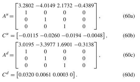
wherek∈N is the current sample, the outputy[mmol/l]stands for the deviation of glycemia from its steady-state value,the inputu[U/min]denotes the deviation of the insulin administration rate from the basal rate,andd[g/min]represents the carbohydrate intake rate input.The state vector of thisnth order model is denotedx[n×1],w[n×1] is the process noise vector and the zero-mean uncorrelated random processv∼N(0,R)represents the measurement noise of the glucose monitoring device[35].

The parameters of model (1) include the state-transition matrixA[n×n],the input matrixB[n×2],and the output vectorC[1×n].The state-transition matrixAconsists of the submatricesAu,Adandthezeromatrices0 oftheconforming dimensions as

where matricesAu[nu×nu] andAd[nd×nd] are in the canonical form and comprise the model coefficientssuch that

The input matrixBis simply

where 0 are the zero vectors of conforming dimensions andBu[nu×1],Bd[nd×1]are equal to

The output vectorCgets

whereCu[1×nu]andCd[1×nd]will comprise the model coefficients as

The state vectorxalso holds the canonical form

wherenuandndare the orders of the corresponding submodels,so the overall model order isn=nu+nd.The state variablesxu,xdrepresent the partial effects of insulin administration and carbohydrate intake,respectively.

Consider that the process noisewin model(1)represents the effect of input uncertainties,so one can write

Since all stochastic terms in(1)were defined as zero-mean uncorrelated stationary random processes, the covariance matrixQ[n×n]of the process noise(9)and the varianceRof the measurement noise are equal to

2.1 State observer

The state vectorxof model(1)is usually estimated using the recursive state observer

where ˆx[n×1] is the estimated state andK[n×1] is the gain vector,which is the subject of the observer design.The design is usually based on the optimal Kalman approach[1,36]in the case of stochastic system assumption,or using the pole-placement method if the system is deterministic.

The state estimate residuale[n×1]will be defined as

Finally,the single step-ahead model output prediction error∊,i.e.the OESO,gets

3 Dynamics of the state observer output error

The model of the state estimate residualecan be derived by substituting ˆx(k+1)from (12) andx(k+1)according to (1a)into(13)while substituting the outputy(k+1)in the terms of 1b as

Eq.(15) can be transformed by applying the forward timeshift operatorzase(k+1)=ze(k)obtaining

The above equation can be reshaped to separate vectore(k)as

whereIis the unit matrix of the conforming dimensions.

According to(14)and(17),∊(k)holds

Eq.(18) implies that the dynamics of the OESO is represented by a stochastic system with multiple independent noise inputs.One may realize that termC(zI-A+KC)-1results in a row vector of rational functionswith the common denominators(z)as the characteristic polynomial of this system.This consideration yields the transfer function model

where

IfQis the covariance matrix of the process noise according to(10),thenw(k)can be written as

where 0 [n×1]is the zero vector,η[n+1×1]is the vector of uncorrelated noise inputs with the unit variance, i.e.,cov(η,η)=I,

whereRis the variance of the measurement noise according to(11).

Finally,model(19)can be generalized as the sum ofn+1 autoregressive-moving-average (ARMA)models by substitutingw(k)in the terms of(21)andv(k)from(23)as

Since the process noise(9)has only two nonzero components and diagonal covariance matrix(10),general model(24)can be reduced to

However, model (24) or (25) cannot be used to predict the OESO,since the random input vectorηas well as the partial outputsare unmeasurable in practice.

Another important paradox concerning this analytical model is that since the covariance matrix of the process noise is considered unknown in the case of suboptimal state estimation,analytical model(24)simply cannot be determined.On the contrary,if the covariance matrix of the process noise is known,what implies that the state estimator works optimally,then model (24) will be known, but it will be unnecessary since the OESO is uncorrelated and hence it cannot be predicted.

Concerning the identification of full model (24) directly from experimental data, i.e.based on the OESO sequence,this would be hardly possible primarily due to its structure and the large number of parameters to be estimated.

The aforementioned issues with predictability and identifiability are the main motivation for further considering two reduced model structures,particularly the autoregressive and the moving average model.

3.1 Optimality test

To test whether the state estimator works optimally or not,the sample autocorrelation function of the OESO sequence has to be analyzed.In the case of optimal state estimation,this autocorrelation function should show a character similar to that of Dirac delta function.

Supposing a finite-length experiment withNsamples,the autocorrelation functionR∊∊(nTs)is estimated as[38,39]

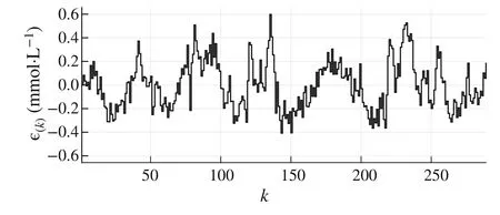
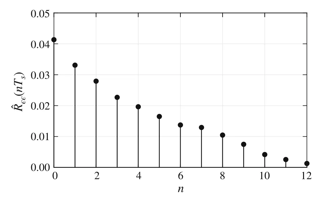
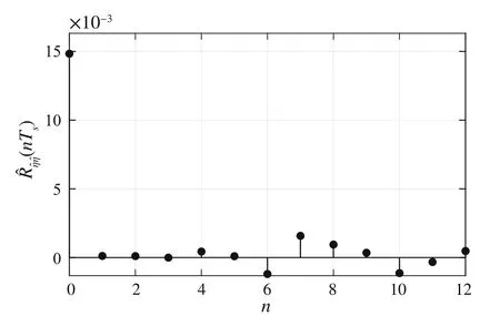
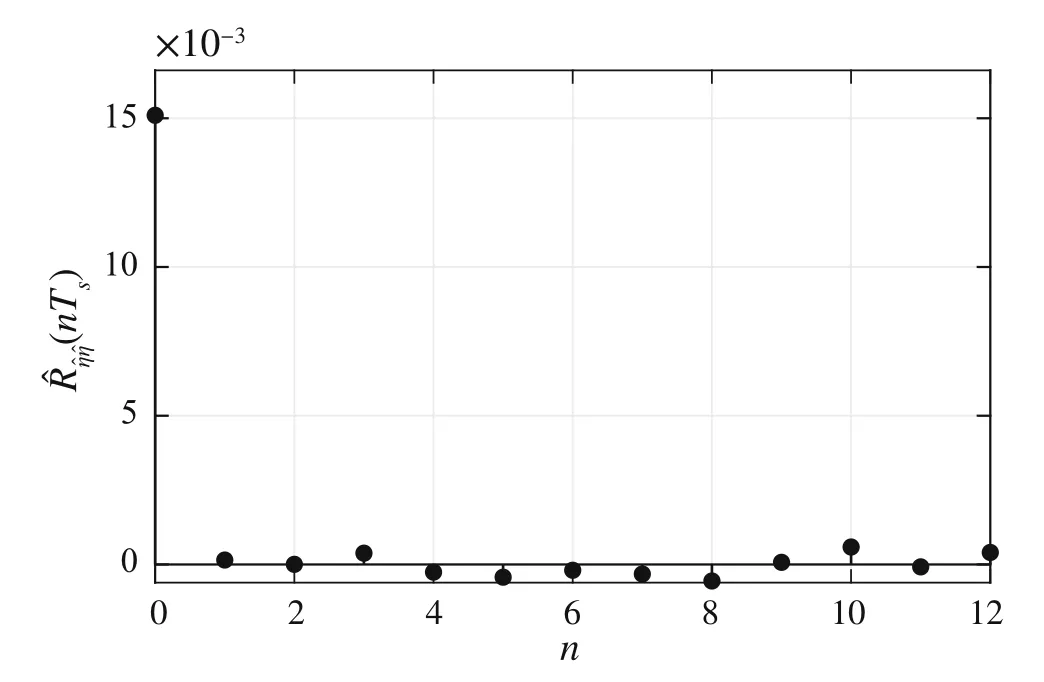
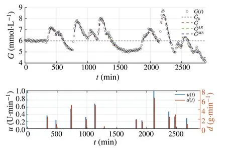
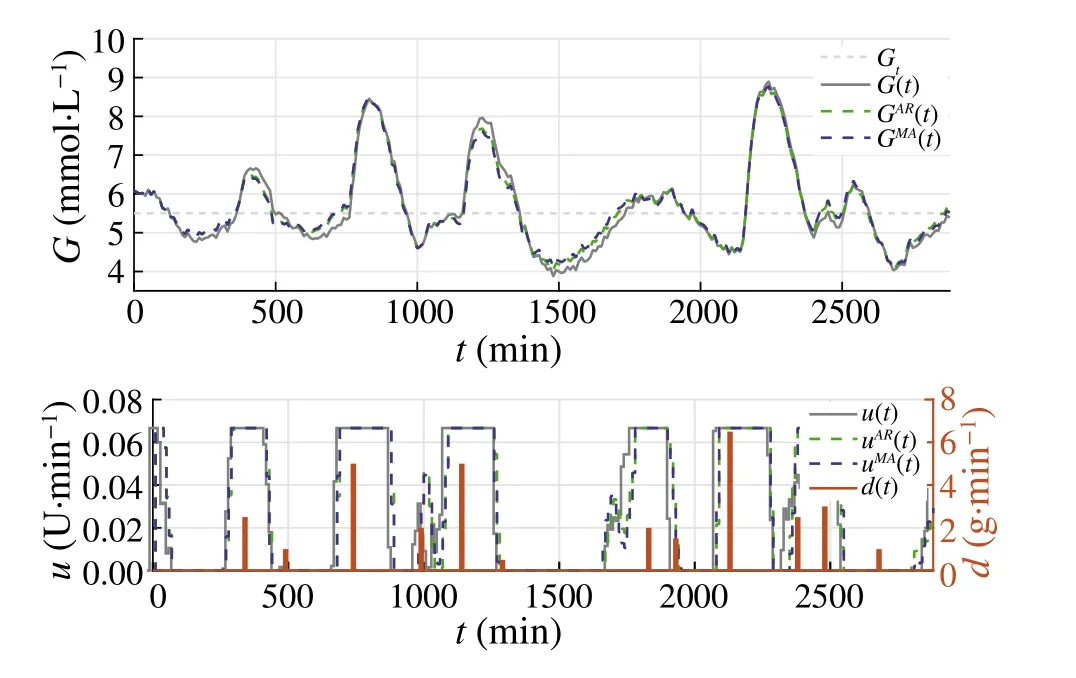
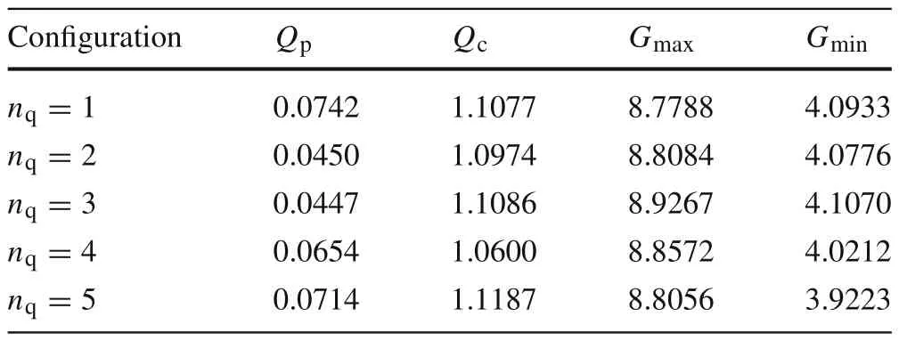
wheren∈Z satisfiesn

4 Autoregressive model

In this section,the dynamics of the OESO will be approximated by the single-input single-output autoregressive model defined as

The polynomialq(z)of thisnqth order model gets

The equivalent difference equation of model(27)holds

The parameter vectorqgets

4.1 Identification strategy

According to difference equation(29),the corresponding linear regression system consideringNavailable samples takes

or using the shorthand notation

whereqis the parameter vector (30),is the regression matrix and∊[N×1],η[N×1]are vectors.

The parameter vectorqcan be estimated as ˆqin a straightforward way using the least squares method with the optimal parameter estimate determined analytically as[40]

4.2 Predictive form

For model(27),the explicit prediction formula can be derived based on difference equation (29).The future values of the whitenoiseinputareobviouslyunknown,soassumingthatits statistically unbiased prediction is zero,i.e.E■η(k+i)■=0,thepredictiveformconsideringthepredictionhorizonnpgets

Sincethenoiseinput in(27)is unmeasurable,byreshaping equation(29),η(k)can be estimated as

5 Moving average model

In this section,the dynamics of the OESO will be approximated by the moving average model

The polynomialg(z)in thength order model(40)gets

The difference equation for model(40)can be written as

5.1 Identification strategy

It is well known that estimating the moving average processes is more difficult than estimating the autoregressive processes[41].Since the input noiseηis unmeasurable in practice,the straightforward approach based on the least squares minimization of the model single step-ahead prediction error cannot be directly applied in this case.

Therefore, to estimate the coefficient vector (43) using the available OESO sequence,the two-step method of Durbin[41,42]will be adopted.The first step of this method consists of fitting an autoregressive model to the OESO sequence via the ordinary least squares method in the terms of Sect.4.In the second step,the identified autoregressive model is used to estimate the input noiseηby filtering the OESO sequence by the inverse of the estimated autoregressive model according to(39).

The second step uses this estimated input noise sequence ˆηto create the regression system and to estimate the parameters of the moving average process in the least squares sense.

The corresponding regression system then gets

or using the shorthand notation,

wheregis the parameter vector(43),is the regression matrix and∊[N×1],η[N×1]are vectors.The optimal parameter vectorgcan be estimated as

5.2 Predictive form

Having the model parameters estimated, the OESO (36)can be predicted.Assuming that the statistically unbiased prediction of the input zero-mean white noise is zero, the predictive form of the moving average model (40) can be derived according to the difference equation(42)as

In practice,the input noiseηcannot be measured,so it has to be estimated based on the inverse filtering of∊according to the difference equation(42)as

6 Prediction and model predictive control with the OESO compensation

In this section,the algorithm of model predictive control will be adopted from[31],while an important modification that concerns the prediction of the OESO will be proposed.

Prediction of the state vectorxand the outputycan be expressed considering(1)as

wherek∈N is the current sample andi∈N getsi=1···np,while assumingnp∈N is the prediction horizon.

Notice that in(52),the OESO ˆ∊,which was predicted by the identified autoregressive or the moving average model,was taken into account by correcting the output prediction ˆy.This is the most important modification of the traditional prediction and predictive control algorithms as it allows us to effectively compensate for the suboptimality of the state estimation.

The predictive control minimizes the quadratic cost function of the model-based predictions of chosen system variables over the prediction horizonnp.The corresponding quadratic form gets[43,44]

whereΔu f[nc×1] is the vector of future changes of the manipulated variable,while assumingncis the control horizon.MatrixA[nc×nc], vectorb[nc×1] and scalarcare defined as

The optimization problem(53)can be solved by quadratic programming if linear inequalities constraints are considered.For the sake of simplicity,the elements of the reference vectoryrare equal to an appropriately chosen constantGtrepresenting the target glycemia.Pursuing the receding horizon strategy, only the first element of the optimal solution

Δu fis actually applied,so one can write

Note that the manipulated variable has to be constrained,so the minimal insulin infusion rateumin=0 U/min, whileumaxwill be adopted from [27].The corresponding linear inequalities system with respect to the decision vectorΔu fcan be formed by involving matrixΨ(57)as in[45]

Compared to[31],the crucial modification of the control algorithm is made here by adding the prediction of the OESO ˆ∊(k+i)to equation(52).

Concerning the safety features of automated insulin therapy, various additional strategies could be considered to enhance the current configuration.To avoid the adverse and dangerous insulin stacking phenomenon,the insulin on board[46–48]representing the amount of insulin still active from the previously administered doses can be involved.The dynamics of insulin on board can be represented by simple linear models like in[49],[50]or[51],while this signal can be used to form a special quadratic penalty that is added to the cost function(53)of the MPC.Alternatively,hard constraints for the insulin on board signal can also be assumed by extending the linear inequalities system(59)of the quadratic program accordingly.Another type of safety feature is to hard constrain the controlled variable by modifying the inequalities system (59) to prevent the risk of hypoglycemia and hyperglycemia as proposed in [26].As this strategy can potentially induce control infeasibility, soft formulation of the controlled variable constraints should be preferred, as proposed in[52,53].However,further details are beyond the scope of this paper.For information on safety features,see,e.g.[46,48,54].Also note that these safety features do not directly interact with the proposed strategy of predicting the output error of the suboptimal state estimator, which is the main contribution of the paper.

7 Experimental setup

To validate the proposed strategy and assess its practical effectiveness in application to the problem of prediction and predictive control of glycemia in subjects with type 1 diabetes, a simulation-based experiment was designed and evaluated.

The glycemia response for this experiment was obtained by in-silico approach, simulating the complex physiologybased nonlinear model that was described in[55,56]and the references therein.The basal state of this model was determined with respect to the basal glycemiaGb=6 mmol/l and the corresponding basal insulin administration ratevb=0.01 U/min.

The orders of empirical model (1) were chosen asnu=nd=4,implying the overall ordern=8.Note that the theory related to estimation of the model parametersin(3)andin(7),is not within the scope of this paper,so we suppose that model(1)was identified with parameters(60).However,for more details on this topic, we refer an interested reader to our recent works[25,57].

Thepredictionhorizonandthecontrolhorizonwereassumed asnp=15,nc=10, while the sample time was chosen asTs=10 min.

The variance of the measurement noise 11 and the variances of the process noise 10 were empirically adjusted as

Note that since the variances of the process noise were just empirically tuned to obtain acceptable performance of the Kalman filter while the actual values cannot be determined because they are not based on any particular physiological mechanisms or characteristics of a diabetic subject,the state estimator will perform only suboptimally in this case, and hence the OESO sequence will be correlated.

The observer gain vectorKwas calculated according to the Kalman filter design[1,36]while considering the model parameters(60)and the noise model parameters(61)as

Concerning the initial tuning of the proposed empirical models of the OESO,the order of autoregressive model(27)was set asnq= 4, whereas the order of moving average model(40)was chosen asng=12.

Fig.1 Evolution of the OESO ∊(k) acquired during the experiment

The experiments were designed to mimic the insulin treatment of a subject with type 1 diabetes during the two-day period.The first investigated problem concerns the prediction of glycemia during standard insulin bolus therapy that wascarriedoutaccordingtotheboluscalculatorrule(see[58]and the references therein).The second deals with automated insulin dosing managed by the model predictive control algorithm of the artificial pancreas.Both algorithms were modified in the terms of Sect.6.

8 Discussion

In this section,the results of the outlined simulation experiment will be comprehensively analyzed and discussed.

The sequence of the OESO obtained in the terms of equation(14)during regular insulin treatment while simultaneously performing the state estimation according to(12)by considering the observer gain (62) is plotted in Fig.1.This figure suggests that although the state estimate asymptotically converges to the actual state,the character of the OESO sequence is far from ideal uncorrelated noise.

To prove this, the autocorrelation function ˆR∊∊of the OESO was estimated according to (26) by processing the sequence from Fig.1 and is plotted in Fig.2.Analyzing this autocorrelation function, one can conclude that the OESO sequence is correlated,what confirms that the state estimator works suboptimally due to the empirically adjusted variances of the process noise(61).

Performing the estimation of both reduced models of the OESO by pursuing the strategies presented in Sections 4 and 5,the following coefficients were estimated.

Parameter vectorqof the autoregressive model(27):

Parameter vectorgof the moving average model(40):

Fig.2 Estimated autocorrelation function ˆR∊∊(nTs) of the OESO sequence from Fig.1

Fig.3 Estimate of the autocorrelation function ˆRˆη ˆη(nTs) of the estimated noise input for the autoregressive model

To validate the models by filtering the correlated OESO sequence∊by the inverse of each of the identified empirical models, i.e.byq(z) and, respectively, the input noise sequence was estimated according to (39) for the autoregressive model and according to (50) for the moving average model.The autocorrelation functions ˆRˆηˆη(nTs) of these sequences for both model structures are depicted in Figs.3 and 4, which show their Dirac delta function-like nature,proving the estimated models valid.

Now follows the prediction of the OESO using the predictive form(34)of the autoregressive model and the predictive form (47) of the moving average model respectively.Relatively accurate predictions for randomly chosen starting points can be observed in Fig.5.Both model structures showed almost identical performances and could predict the future evolution of the correlated OESO with a satisfying accuracy considering the highly stochastic nature of this signal.

Fig.4 Estimate of the autocorrelation function ˆRˆη ˆη(nTs) of the estimated noise input for the moving average model

Fig.5 Prediction of the OESO using the both autoregressive model)and the moving average model

The next comparison concerns the practical impact of correcting the glycemia prediction by predicted OESO as the original contribution of the paper.In Fig.6,one can see the uncorrected prediction of glycemia(ˆG)as the conventional strategy,as well as the predictions that involved the corrections by OESO predicted using the autoregressive(ˆGAR)and the moving average(ˆGMA)model.By a basic visual assessment, one can observe an improvement of the prediction accuracy, while the improvements concerned primarily the peaks of the response.Keep in mind that such differences between the uncorrected and the corrected prediction can be critical in situations such as decision making with regard to the application of insulin therapy.

In addition to the graphical assessment,the prediction performance will be quantified by the quadratic metric

which will provide a better assessment of the prediction performance.

The last part of the experiment is focused on the model predictive control of glycemia in the context of the artificial pancreas implementation,where a positive effect of the proposed predictors on control performance is anticipated.To demonstrate this,Fig.7 shows the closed loop glycemia response,where involving the predictions of the OESO visibly improved the control performance in terms of tighter control with respect to the reference value, and reduced maximal and minimal observed glycemia,what is especially significant to reduce the risk of hyperglycemia and hypoglycemia.It can be concluded that both predictors performed almost identically, but way better than in the original case without compensating for the OESO.

Fig.6 Prediction of glycemia without the OESO compensation G(t)compared to using the autoregressive model GAR(t) and the moving average model GMA(t)

Fig.7 Predictive control of glycemia without the OESO compensation G(t)compared to using the autoregressive model GAR(t)and the moving average model GMA(t)

Keep in mind that since typical values of the OESO are relatively low compared to the magnitude of the controlled variable(see Fig.1),the proposed strategy can naturally yield a limited effect.It can also be claimed that the strength of the desired effect is directly related to the performance level of the state observer and thus to the degree of mismatch between the process noise model and the actual statistical properties of the system.Therefore,for systems with an empirically tuned covariance matrix of the process noise,the strategy proposed in this paper is highly recommended.

The control performance will be quantified by the maximalGmaxand the minimalGminobserved glycemia,and by the quadratic metric

Table 1 Comparison of the prediction and control performance metrics

Table 2 Comparison of the prediction and control performance metrics for the autoregressive model

Table 3 Comparison of the prediction and control performance metrics for the moving average model

whereGtis the target glycemia.

The summary of prediction and control performance metrics obtained during the experiment is documented in Table 1,which also confirm the observations from Figs.6 and 7.

Toinvestigatetheeffectofthechoiceofthetunableparameters of the OESO models, particularly the order of the autoregressive model (27)nqand the order of the moving average model (40)ngon the resulting performance of the proposed strategy, the experimentation was repeated under various configurations, yielding the results summarized in Tables 2 and 3.

It can be concluded that the moving average model of the OESO performs slightly better in both prediction and predictive control than the autoregressive model,while the choice of the corresponding model ordersnq,ngalso affected the overall performance,yet not consistently for all the metrics considered.However, all studied models performed better than the original uncompensated configuration.

9 Conclusions

This study stressed that the OESO sequence in the case of suboptimal state estimation is correlated, while it can be effectively predicted by the autoregressive or the moving average models.These two reduced models could provide good predictability and identifiability from the experimental data.The predicted OESO was then involved to correct the output variable prediction and hence ultimately improve the performance of the model predictive control.It can be concluded that the presented strategy allowed to effectively compensate for the suboptimality of the state estimation caused by the inaccuracy of the process noise model in a relatively inexpensive and feasible way.

We also obtained theoretical results demonstrating that the actual dynamics of the OESO is analytically described as the sum of ARMA processes,while this full structure was approximated by the autoregressive and the moving average models in practice.

A promising application of our results would be possible within an implementation of the artificial pancreas in subjects with type 1 diabetes,where maximizing the performance of the model predictive control is of highest priority.The presented simulation-based experiment demonstrated that the dynamics of the OESO can be effectively predicted by both proposed reduced models,while there were documented positive effects on the accuracy of the glycemia prediction and on the performance of the predictive control.Keep in mind that although qualitative improvements do not appear to be significant at first sight,any feasible improvement matters a lot when managing glycemia and can have significant longterm consequences for patient health.

Compared with the conservative structure of the MPCbased artificial pancreas[6,32–34]that utilizes the Kalman filter state estimation with typically empirically tuned covariance matrix of the process noise,which normally results in its suboptimal performance,the strategy proposed in this paper additionally involves an easily identifiable prediction model of the OESO to effectively compensate for the adverse effect of suboptimality of the state estimation by correcting the system free response prediction.Moreover, this structural modification is not computationally demanding and it can be easily embedded to the existing modular MPC schemes[6, 32–34] without involving any hardware adjustments or directly interacting with other features of the artificial pancreas such as constraints.

On the contrary, compared with the alternative solution based on methodological estimation of the covariance matrix of the process noise according to the methods presented in[18–22]to implicitly ensure the optimality of the state estimation,it can be claimed that these methods typically require very large experimental datasets(tens of thousands of samples)to provide reliable and unbiased estimates,whereas the statistical models of the OESO proposed in this paper can be identified from relatively limited experimental data(hundreds of samples).

In a nutshell,the most significant contributions presented in this work include the derivation of the analytical stochastic ARMAmodeloftheOESOanditsapproximationswhichcan be used to improve the performance of the suboptimal state observer in applications when the process noise model is not exactly known or is uncertain.It can be concluded that the actual effect of the proposed strategy depends primarily on the degree of plant-model mismatch of the noise model.

Funding Open access funding provided by The Ministry of Education,Science,Research and Sport of the Slovak Republic in cooperation with Centre for Scientific and Technical Information of the Slovak Republic Open access funding provided by The Ministry of Education,Science,Research and Sport of the Slovak Republic in cooperation with Centre for Scientific and Technical Information of the Slovak Republic.

Declarations

Conflict of interest The authors have no competing interests to declare that are relevant to the content of this article.

Open Access This article is licensed under a Creative Commons Attribution 4.0 International License,which permits use,sharing,adaptation, distribution and reproduction in any medium or format, as long as you give appropriate credit to the original author(s) and the source, provide a link to the Creative Commons licence, and indicate if changes were made.The images or other third party material in this article are included in the article’s Creative Commons licence,unless indicated otherwise in a credit line to the material.If material is not included in the article’s Creative Commons licence and your intended use is not permitted by statutory regulation or exceeds the permitteduse,youwillneedtoobtainpermissiondirectlyfromthecopyright holder.To view a copy of this licence, visit http://creativecomm ons.org/licenses/by/4.0/.