Motion simulation of moorings using optimized LSTM neural network*
2023-11-10ZhiyuanZHUANGFangjieYUGeCHEN
Zhiyuan ZHUANG, Fangjie YU,2,**, Ge CHEN,2
1 Department of Marine Technology, College of Information Science and Engineering, Ocean University of China, Qingdao 266100, China
2 Laoshan Laboratory, Qingdao 266237, China
Abstract Mooring arrays have been widely deployed in sustained ocean observation in high resolution to measure finer dynamic features of marine phenomena.However, the irregular posture changes and nonlinear response of moorings under the effect of ocean currents face huge challenges for the deployment of mooring arrays, which may cause the deviations of measurements and yield a vacuum of observation in the upper ocean.We developed a data-driven mooring simulation model based on LSTM (long short-term memory) neural network, coupling the ocean current with position data from moorings to predict the motion of moorings, including single-step output prediction and multi-step prediction.Based on the predictive information, the formation of the mooring array can be adjusted to improve the accuracy and integrity of measurements.Moreover, we proposed the cuckoo search (CS) optimization algorithm to tune the parameters of LSTM, which improves the robustness and generalization of the model.We utilize the datasets observed from moorings anchored in the Kuroshio Extension region to train and validate the simulation model.The experimental results demonstrate that the model can remarkably improve prediction accuracy and yield stable performance.Moreover, compared with other optimization algorithms, CS is more efficient and performs better in simulating the motion of moorings.
Keyword: mooring; motion simulation; long short-term memory (LSTM); optimization strategy; hybrid deep learning
1 INTRODUCTION
The moorings, as a vital part of ocean observation equipment, can be anchored at a fixed location and carry various sensors for gathering long-term,sustainably, and multi-parameters in-situ measurements(Venkatesan et al., 2018; Zhang et al., 2021b).Meanwhile, the cooperation of mooring arrays has been widely applied both in providing more complete spatiotemporal data and measuring finer dynamic features of marine phenomena (McPhaden et al.,2009; Liu et al., 2018).The measurements of concurrent temperature/salinity and velocity obtained from mooring arrays detail analyze the dynamic features of subthermocline eddies in the Kuroshio Extension region (Zhu et al., 2021).The data from the array with five moorings deployed near Mackenzie Canyon,Beaufort Sea clarified the components and variability of the boundary current system (Lin et al., 2020).
However, the moorings easily experience irregular vertical displacement under the effect of ocean currents and generate nonlinear responses due to the various components of the mooring are connected by a flexible cable (Zhao et al., 2013).The highly unstable movement may yield huge deviations in the observations from the following aspects: the actual observation depths are not consistent with the planned,which can generate huge errors in the measurements of the ocean parameters with significant vertical gradients (temperature etc.); and the position of the instrument anchored in the top of the mooring cable will decrease, which may produce the vacuum of top-level observation.This largely affects the spatial integrity and accuracy of the observations and further determines the deployment of the mooring array.Furthermore, it is a prohibitive cost to perform largescale operations with mooring arrays (Clark et al.,2020; Zhao et al., 2020).
Recognition of the above, quite a few studies are focusing on the movement of the moorings.Based on the potential flow theory, Aamo and Fossen (2001)developed a finite element mooring cable model to study the dynamics of moorings.However, the model ignored the high ductility of the cable under the ocean currents that makes the model unstable.To overcome the above issue, Montano et al.(2007)proposed a new mixed finite element method and designed an anchored buoy dynamics simulation program for the mooring with elastic cables.Besides, to study the attitude control and dynamical characteristics of moorings, the fluid model is constructed by thorough considering the elastic deformation of the mooring cable and the current resistance from tangent and normal (Wang et al.,2012).Ge et al.(2016) also presented an attitude control law of the mooring based on the strong nonlinearity of the mooring space motion.The establishment of motion models often brings complex calculations of control equations, Ge et al.(2014) and Qui et al.(2013) utilized the lumped mass method to obtain the movement elements and attitude change of moorings which through avoiding the derivation of partial differential equations in the control of buoys to ease the difficulty of the model.However, the study only validated the dynamic response of mooring in static situations.Wang et al.(2019) also designed the dynamic model of the submerged buoy with the lumped mass method and analyze the response of the submerged mooring system in different flow velocity conditions.Aiming at the nonlinear responses of the mooring, the study of Ma et al.(2016) established a mooring motion numerical model and further revealed the remarkable nonlinearity and the sub-harmonic response of the mooring motion affected by the time-varying rope tension.In recent years, many scholars began to introduce the idea of artificial neural networks(ANN) into the study of moorings.Zhao et al.(2021) combined BP neural network with the finiteelement method (FEM) to realize the prediction of the statistic pretension and dynamic tension series of moorings under complex ocean states, considering multi-parameters including the azimuth, the length of the mooring ropes and the radius of moorings.Qiao et al.(2021) introduced the idea of LSTM(long short-term memory) into the research on the internal turret FPSO (floating production storage and offloading) and constructed the LSTM-based prediction model to study the mooring line tension prediction under given sea states, in which the ship motion signals are set as the inputs, the dynamic mooring lines responses are outputs.Based on the above study, Li et al.(2022) performed the FPSO prediction research under the irregular wind, wave,and current directions conditions based on LSTM neural network.Then a new mooring line tension prediction approach is proposed, in which the input data is the 6-DOF (degrees of freedom) motion of the equipment while the output labels are distinguished into the corresponding low-frequency and wavefrequency responses of moorings (Wang et al.,2022b).Furthermore, Yao et al.(2022) targeted mooring system damage detection and established the PCA-LSTM model, which effectively integrates the motion prediction model with the anomaly detection model.
To summarize the methods and techniques used above, they can more or less predict the mooring motion and improve the movement stability by studying the motion law of moorings, but the main targets of these studies are the hydrodynamic response and the mechanical model of the mooring system.With the operation of moorings is moving towards the deep-sea, the scale and time resolution of measurements is increasing, as well as the complexity of working scenery, the existing studies are not fully feasible to capture and utilize the nonlinear features of the motion of moorings to build models quickly and improve the accuracy of prediction.Bearing the above in mind and further improving the motion prediction accuracy, we design a completely datadriven mooring simulation model in this paper,considering multiple factors, which can directly learn motion discipline from the training data to perform prediction, without any prior.Based on the accurate predictive information, we can conduct the correction of the observations, assimilate the data from heterogeneous and non-synchronized sensors,monitor the running of the mooring units, and further provide reference methods for the control of mooring arrays.Considering high time resolution and temporal continuity of the observation data of moorings, the model adopts the LSTM neural network, which can avoid the long-term dependence of time-series data as the bracing algorithm to solve the mooring motion prediction problem.Note that the LSTM neural network architecture is of great importance in the prediction accuracy and generalization, the cuckoo search (CS) optimization algorithm is applied to optimize the LSTM neural network parameters.The CS is derived from the reproduction strategy of cuckoos and the pattern of levy flights, which mainly mimics the process of searching for an optimal nest to hatch the eggs through random wandering to solve the optimization problem.Compared with other optimization algorithms, the parameters of the CS algorithm are less which leads to a faster convergence speed and higher calculation accuracy.The experimental results demonstrate that the proposed CS-LSTM model offers superior optimization performance, stability,and robustness.
The following structure of this paper is organized as below.An introduction of the dataset is shown in Section 2.The related materials and methods are stated in Section 3.In Section 4, we give a comprehensive presentation of the results of the experiments as well as the discussion.Finally, Section 5 summarizes the conclusions.
2 DATASET
Not only appropriate deep learning algorithms can prominently improve the performance of the simulation model, but the relatively accurate measurements are also of great importance.Three sets of in-situ observation data collected by three moorings anchored are employed to train and test the simulation model.The instruments were deployed in the north-western Pacific Ocean from October 2017 to May 2018(marked as triangles in Fig.1b), lasting a 7-month period of continuous measurements.The background of Fig.1b is sea-level anomalies where the stronger the anomaly signals, the greater the possibility of the existence of the ocean dynamic process.As we can see from the composition of the mooring presented in Fig.1a (here we take M2 as an example because only the tethering positions of the sensors are different in other instruments), one complete full-depth mooring system consists of three RCMs (recording current meters), four CTDs (conductivity, temperature, depth),and one ADCP (acoustic Doppler current profiler).The RCMs were used to acquire a single layer of temperature and horizontal velocity and the ADCP recorded current velocity profiles over a range of 600 m with a 10-m spatial scale.Furthermore, the motion of the mooring is observed according to the adjustment of the position data calculated from the pressure sensors within CTDs.Hereby, the mooring motion series is formed by coupling in-situ ocean current data (observed by ADCP or RCMs) and position data (deriving from CTDs) at different depth layers.Figure 1c–e presents the motion sequence of layer 1 in M1, M2, and M3, respectively.We can find that the datasets not only have significant time continuity but also exist obviously unstable behaviors and steady periods.The sampling interval for RCMs and ADCP was set as one hour (the minimum sampling rate of sensors), which is twice that of CTDs.To ensure the sustainability of long-term observation and consistency of time resolution for multi-source data, we checked the data and finally determine the time resolution of the datasets as one hour.Moreover, it is worth noting that the current data observed by ADCP exist certain not a number(NAN) value or empty value owing to the current measurement principles of ADCP (utilizing the principle of acoustic Doppler effect to measure flow velocity) and the current characteristics.Considering the high spatiotemporal resolution of the observations, these errors, however, are negligible.Furthermore, we have introduced nearestneighbor interpolation method or replacing these values with the surrounding values when performing data pre-processing and constructing the motion series.Other parameters of the moorings are shown in Table 1.

Table 1 The parameters of the mooring system
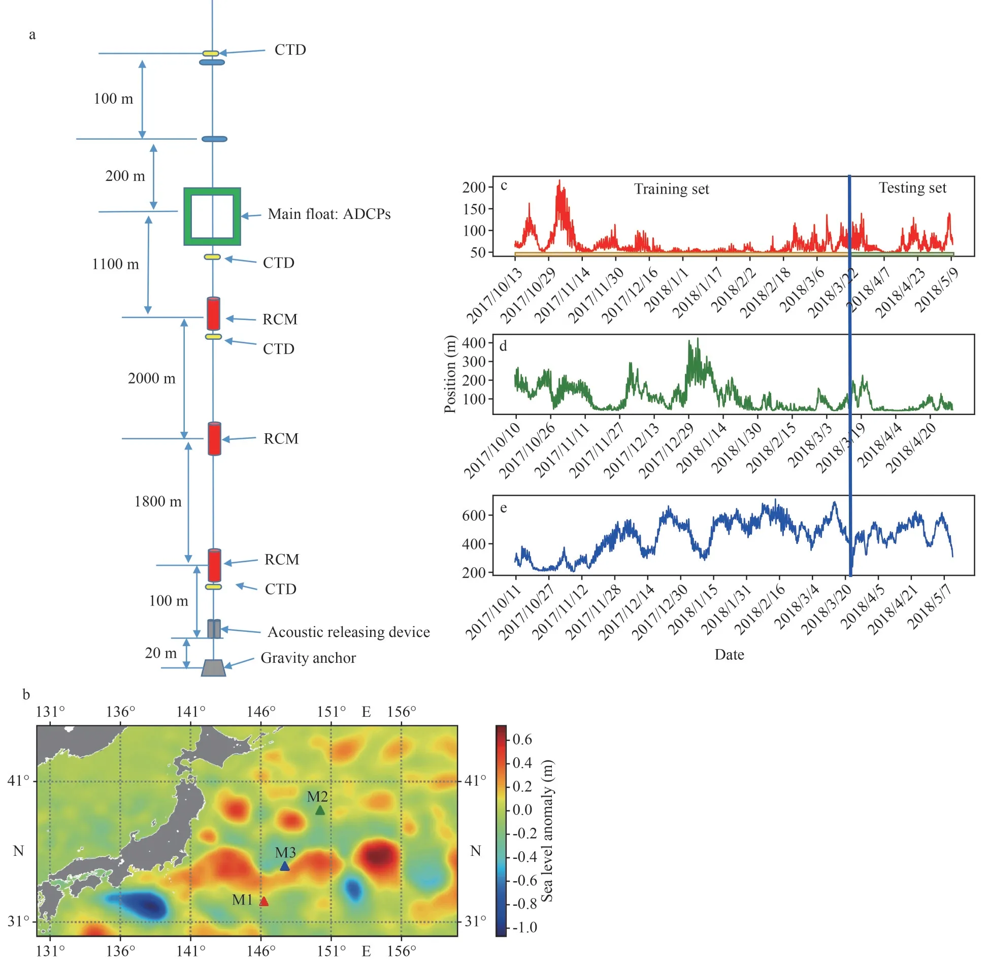
Fig.1 The approximate deployed area and motion time series of moorings
3 RELATED METHODOLOGY
In this section, we formally introduce the simulation framework together with the materials and methods we adopted in this paper.The flow chart is shown in Fig.2.
3.1 Overview of the framework
Figure 2 presents the technique flow chart of our research.It is obvious including three parts: constructing the mooring motion series by combining the real-time ocean current and position dataset; training the model,and testing the model.In order to improve the performance and robustness of the simulation model,we introduce the cuckoo search optimization algorithm to tune the hyperparameters of the LSTM neural network.Meanwhile, we design several comparative experiments to further validate the effectiveness of the model and we conducted an exploration of mooring long-sequence prediction.
3.2 LSTM neural network
The LSTM neural network is one variation of the recurrent neural network which was first proposed by Hochreiter and Schmidhuber (1997).It not only inherits the ability of Recurrent neural networks(RNN) to capture the temporal dynamics of time series data but also can solve the gradient vanish or explosion of RNN effectively (Li et al., 2019).The key that LSTM achieving the above abilities is the introduction of cell state (ct) based on RNN.The cell state receives the information generated in earlier time nodes according to three gate units, respectively forget gates,input gates, and output gates (Fig.3) (Zhang et al.,2020).Taking the dataset of a certain observation point as an example, the working principle of the three gate units and cell state is shown as follows:

Fig.2 The proposed algorithms for mooring motion simulation
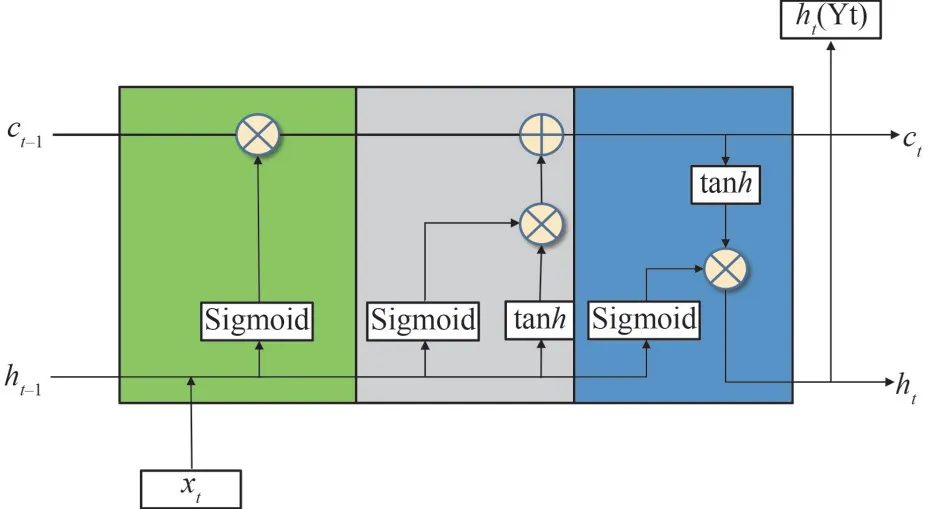
Fig.3 The structure of long short-term memory (LSTM)neural network
The symbol indicates:W,Uare the weight matrices,bis the offset generated in the process from the input gate to the output gate, which is calculated during the training of the model,xtis the input current and position at the current timet,htis the corresponding output position at the current moment,ht–1is the corresponding output position of the input value at the previous moment, andσis the activation function sigmoid which scales the input value to [0,1] (0 denotes the information is completely abandoned and 1 represents that completely reserved).
Step 1: the LSTM decides what information will be discarded from the previous cell state, theftdenotes the forget gates:
Step 2: the LSTM determines what new information is added to the cell state:
Theitis the input gates that decide what information needs to be updated and thec~tdenotes the candidate value to be updated.
Step 3: the final cell statectis updated based on the output values from forget gates and input gates.
Step 4: the LSTM determines the output valueht(Yt) with the output gatesot:
3.3 Optimization strategy
3.3.1 Dropout regularization
Dropout is a classic regularization method that is of great importance in alleviating the overfitting of neural networks (Srivastava et al., 2014).The dropout operation refers to randomly dropping neurons at a specific ratio during the training stage of the network, which avoids the performance of the model having an over-reliance on certain features(Krizhevsky et al., 2017).We introduce the dropout mechanism into the training of LSTM, which not only eases the complicated structure of LSTM but also improves the robustness of the model.
3.3.2 LSTM neural network architecture optimization strategy
Even though LSTM has many superior features we can learn from the above and we have adopted dropout regularization to enhance the stability, the performance of the LSTM algorithm is strongly affected by the multi-parameters defined by researchers in practical applications (Wei et al., 2020).The involved parameters of the LSTM neural network comprise the sequence length (SL), the learning rate(LR), the dropout ratio (DR), the number of LSTM layers (LLN), the number of neurons of LSTM layers(LLNN), the number of full connection layers (FLN),and the hidden neurons of full connection layers(FLNN), etc.Therefore, it is significant to determine how to find the optimal hyper-parameters construction.In this paper, we choose the above hyper-parameters as the optimization objects which have great influences on the performance of LSTM.Some other default hyper-parameters are shown in Table 2.
In the early researches of optimization algorithms,the grid search algorithm plays an important role(Kong et al., 2017).However, it has some shortcomings in optimizing high-dimensional spaces and many complex network configurations such as computationally expensive (Jiang et al., 2013).Many studies proved that the random search process is more efficient (Bergstra and Bengio, 2012) and several intelligent optimization algorithms are proposed.In our study, we introduce cuckoo search optimization algorithm to find the optimal hyperparameters of LSTM.The following sections will present how the method works.
3.3.3 Cuckoo search optimization method
The cuckoo search optimization is a natureinspired heuristics optimization algorithm based on the brood parasitism behavior of the cuckoo bird,and was introduced by Yang and Deb (2009)(Bhargava et al., 2013).The levy flight method is used in CS for performing effectively in the global search and the local search to obtain the optimal solution, which avoids being trapped in local optimization when performing LSTM parametersoptimization.The parameters of CS are less than that of classical optimization strategies such as genetic algorithm (GA) and the particle swarm optimization (PSO), which contributes a faster convergence.Furthermore, the application of CS algorithm is not widespread.The process of utilizing the method to select the best parameters of LSTM(SL, LR, DR, LLN, LLNN, FLN, and FLNN) can be described as follows and the schematic of the optimization algorithm is shown in Fig.4:
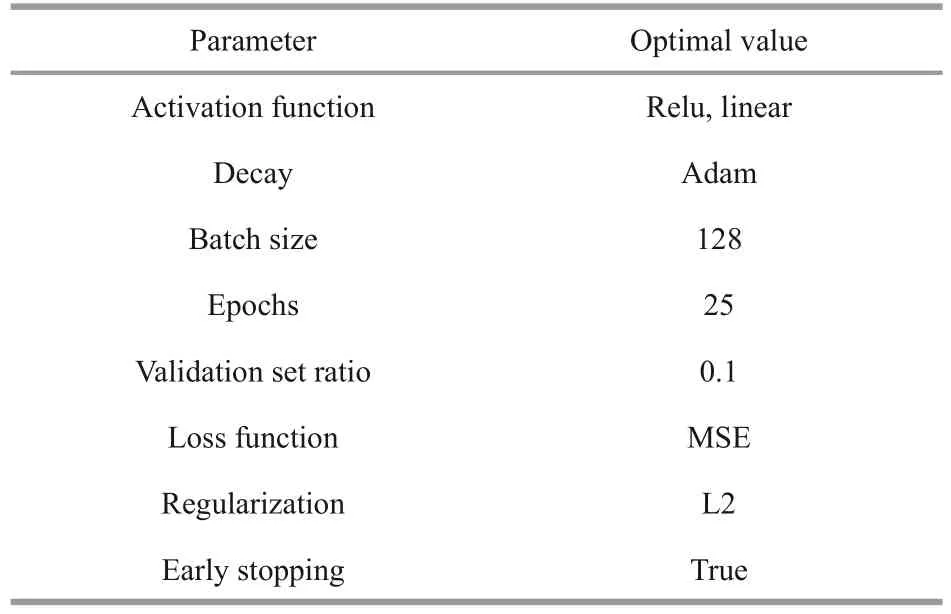
Table 2 Some other default hyper-parameters of LSTM
(1) Nest initialization: the parameters to be optimized in LSTM are combined to generate the initial nests.The number of the nest is set as 20 and the iteration steps are 20.
(2) Fitness evaluation: the parameters of each nest are used to construct the mooring motion model.The performance of the nest is calculated by the fitness function (mean square error).The nest with the minimum fitness value is selected as the best result.
(3) Updating the nest: introducing the levy flight mechanism to generate random values to update the nest (the details of levy flight can see Yang and Deb(2009)).The fitness of each nest is recalculated and the best solution can be updated.
(4) Abandoning the nest: setting the probability(pa) that the nest will be abandoned to further update the nest.Recalculating the fitness to select the best nest.
(5) Repeating the workflow from (2) to (4) until achieving the best solution.
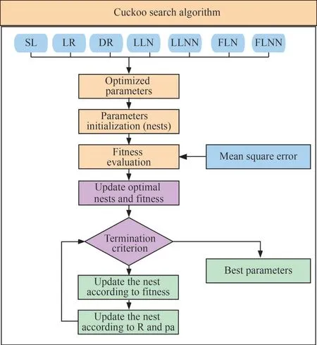
Fig.4 The schematic of the optimization algorithm
The CS parameters mentioned above are shown in Table 3.
4 RESULT AND DISCUSSION
In this section, we conduct several experiments to validate and evaluate the accuracy and efficiency of the algorithms mentioned above.We employ the mooring datasets to perform the case study.In our study, the whole moving process of the mooring is described as the datasetS={(xi,yi)}.xi=[Vi,Di] whereVidenotes the velocity observed by ocean current meters andDirepresents the depth position of mooring atithtime point.yiis the depth of mooring atithtime point.The datasets are divided into different layers (the data in layer 4 of M3 is lost during the observation) according to the data acquisition range of the sensors.Meanwhile, the raw datasets are reconstructed in the form of {(x1,x2,…,xn,yn+1), (x1,x2,…,xn,yn+1,…,yn+t)} (Fig.5) and are divided into two parts: the training set and the testing set.Considering this is long-time series predictionresearch and to keep the integrity of the motion information, the shuffling mechanism is not applied.The first 75% of each dataset (approximately the dataset observed from October 2017 to March 2018)is applied as the training set for model training and parameters selection.The rest 25% (roughly the dataset from March 2018 to May 2018) are selected as the testing set to testify the prediction capabilities.The detailed division is shown in Fig.1c–e where blue solid line marks the division of training set and testing set.Two parts are distinguished by different colors and fully considered the stable and unstable periods of datasets.The design of the experiments is shown in Table 4, the datasets and the optimized variables in the experiments are identical.
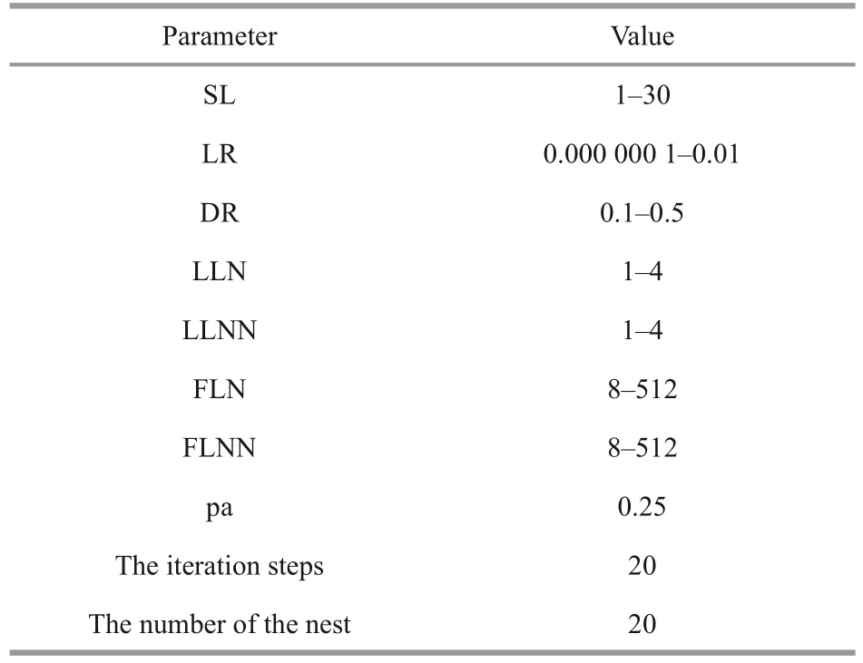
Table 3 The values of parameters
The experiments can be divided into two parts,including single-step prediction and multi-step prediction.The meaning of single-step prediction is using historical time series [x1,x2,…,xn] to predict the next time series [yn+1] , the meaning of multi-step prediction is using historical time series [x1,x2,…,xn] to predict the nextt-step sequence [yn+1,…,yn+t].In our study, the input and output can be described in Fig.5.
The pivotal idea of the experiments is using the past several hours (determined by the hyper-parameters SL) current and position information as the initial inputs to forecast the location of the mooring in the future time steps and minimize the deviation between the observed values with the predicted values.
4.1 Normalizing the dataset
Normalization has been widely introduced in data pre-processing to map the values of different defined fields to the same interval uniformly to eliminate the adverse effects caused by abnormal sample data.In this paper, we adopted the normalization function of Min-Max Normalization to scale the input multi-dimensional training data.The formula is shown as follows:
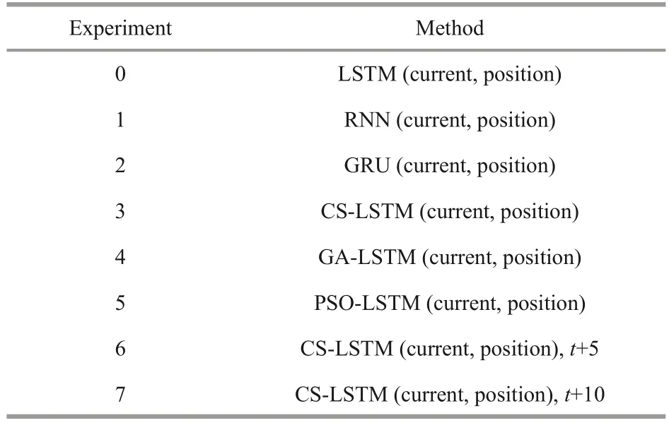
Table 4 The design of experiments
wherexis the original position and current,Xnormis the normalized value,Xmaxis the maximum value of input training data, andXminrepresents the minimum value of input training data.
4.2 Performance evaluation
The assessment results will be shown in this subsection, which is divided into three parts.Firstly, we design experiments 0–3 to carry out the comparative analysis for figuring out the performance of the simulation model.Secondly, experiments 3–5 are used to verify the performance of the optimization algorithm in tuning parameters of LSTM.Experiments 6–7 are used to explore the performance of multistep prediction based on our proposed model.Lastly,we further validate the time-consuming and convergence of the proposed optimization models.
4.2.1 Comparative analysis with mainstream algorithms The Recurrent neural network (RNN), Gated recurrent unit (GRU), and LSTM are three typical time-series research models, which all can calculate the future data by remembering the data from the previous moment (Che et al., 2018; Perumal et al.,2021; Zhang et al., 2021a).The RNN, the versatile tool for time series applications, is the prototype of LSTM that can perform time sequence prediction based on the time series characteristics of input variables (Wang et al., 2022a).The GRU is a variant of LSTM architecture, consisting of the update gate and reset gate to achieve time-series predictions(Irrgang et al., 2020).Therefore, we employed them as baselines to conduct comparison experiments to verify the performance of the proposed models.In these comparison experiments, the LTSM hyperparameters in Experiment 0 are manually tuned and the values are set as 20, 0.001, 0.3, 2, 128, 64, and 164.The hyperparameters of RNN and GRU are consistent with CS-LSTM, which are optimized in the training process.As shown in Figs.6–8, the predicted motion trajectories of three moorings adopting different models are plotted together with the observed values.To demonstrate clearer and distinguish the detailed difference, we further added the corresponding partial zoom-in graphs.As we can see from the figures, the real motion series of different layers of each mooring is generally consistent and has an obvious distinction between strong and weak motion signals.Compared with the real trajectories, major of the results from the baselines have a great tendency of right-shifter.Meanwhile, the results demonstrate that the benchmarks only have a great performance in predicting the motion series with strong signals.However, for the proposed model, the predicted curve (orange) is generally in keeping with the in-situ observations (black), without a conspicuous phase difference and the movement trend of the weak signals in the motion series can be effectively captured.
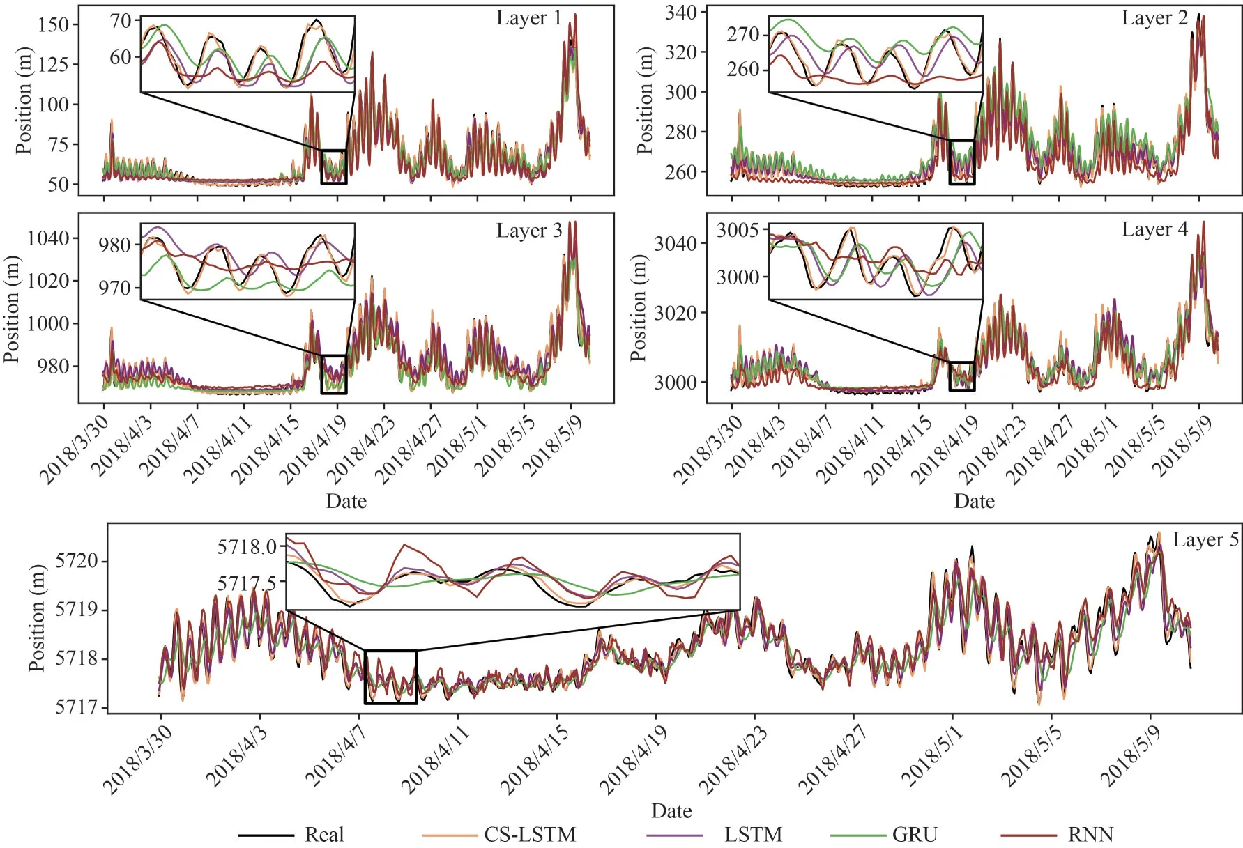
Fig.6 The comparison of the forecasted motion trajectory of the M1 by several algorithms with the observed trajectory

Fig.7 The comparison of the forecasted motion trajectory of the M2 by several algorithms with the original trajectory
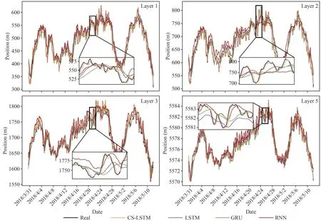
Fig.8 Comparison of the M3 motion trajectory reconstructed by several algorithms with the observed values
Based on the simulation information of the proposed models and other comparative baselines,we can quantitatively assess the simulation accuracy by introducing performance criteria.As far as we all know, there is no unique method and consistent standards to verify the effectiveness and stability of the simulation results and the single metric rule cannot fully explain the characteristics of the model.In this paper, we adopt composite evaluation methods, including MAE, RMSE, andR2as listed in Table 5.TheNrepresents the quantity of the dataset,yrealis the real position, andypreddenotes the predicted position.Figures 9–11 show that the performance of the proposed models has great improvements over other models, which can replicate better results with the lower MAE and RMSE and higherR2(press close to 1).
We can also find out that the simulation performance has a different level of performance in each layer, with the tendency to gradually advance as depth increases.We think that the different strengths of the ocean current at different depths play an indispensable role, where the flow field in the upper ocean is confirmed more intense (Cenedese and Gordon, 2021).
4.2.2 Research and exploration of multi-step prediction
Multi-step prediction is also known as long-term prediction, which means, as mentioned above, using the historical time series to forecast the followingtstep sequence.The key strategy of multi-step prediction is consistent with the single-step: traverse the data according to the time steps determined by SL and divided the data into overlapping windows,advance one-time step in each iteration, and predict the position of mooring for multiple consecutive time steps including the target time point.
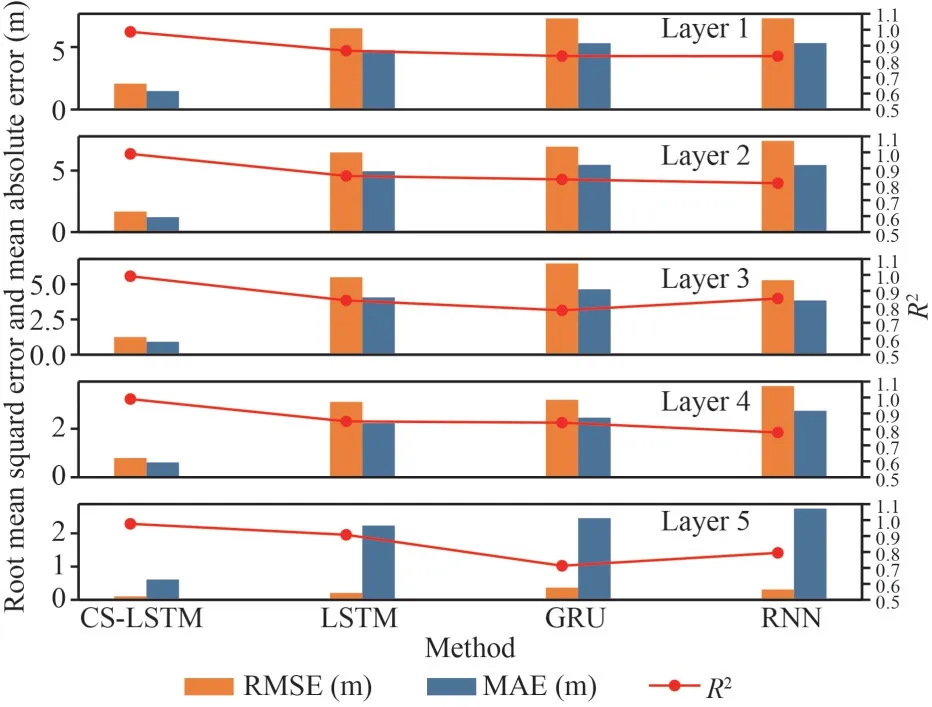
Fig.9 Comparison of RMSE, MAE, and R2 values of related models of M1
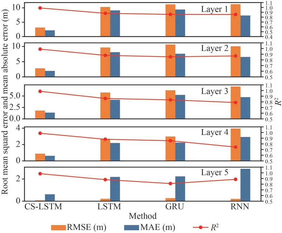
Fig.10 Comparison of RMSE, MAE, and R2 values of related models of M2

Table 5 Performance evaluation rules

Fig.11 Comparison of RMSE, MAE, and R2 values of related models of M3
The multi-step adds the continuous change information of the mooring motion compared with single-step prediction, which is of great significance to the study of mooring long-term motion characteristics and the capture of motion trends.We make multistep experiments oft+5 andt+10 based on the proposed model to conduct explorations on the long sequence prediction of the model.The results are shown in Figs.12–13.We can find that CS-LSTM can also achieve good accuracy in makingt+5 andt+10 predictions and demonstrates the same characteristic as the single-step prediction from the following aspects: a) the predicted performance is increasing with the depth; b) the effectiveness of the model applied in M1 and M2 is better than that in M3,which confirm that the rationality of the conclusion we draw in single-step prediction.Besides, the prediction accuracy of the proposed model is decreasing with the increase of the prediction time step where the singlestep prediction has the best accuracy, thet+5 is second and thet+10 prediction has the worst preciseness.4.2.3 The evaluation of the optimization of LSTM
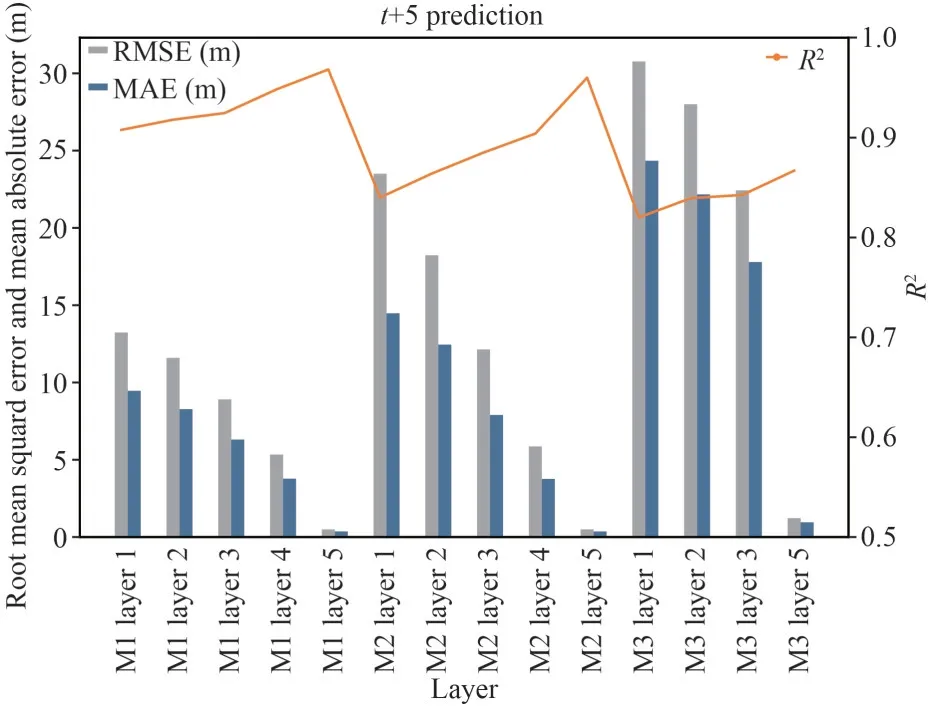
Fig.12 Comparison of RMSE, MAE, and R2 values of proposed models in (t+5) prediction
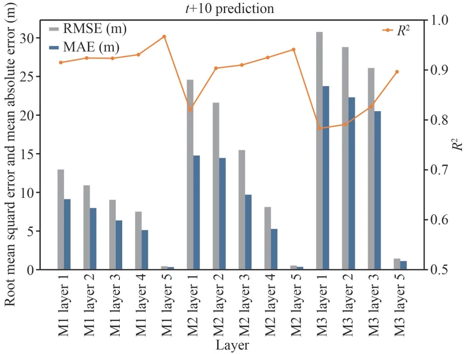
Fig.13 Comparison of RMSE, MAE, and R2 values of proposed models in (t+10) prediction
From the above discussion, the accuracy, and the effectiveness of the proposed models have been confirmed, in this subsection, we validate the optimization performance of the CS algorithm by introducing two classic optimization algorithms,including the genetic algorithm (GA) and the particle swarm optimization (PSO).The Genetic Algorithm is a search algorithm based on natural selection and group genetic mechanisms.Through simulating the phenomenon of reproduction, hybridization, and mutation in natural selection and natural genetic process to obtain the optimal solution (Oliveri and Massa, 2011).The Particle Swarm Optimization is a heuristic algorithm to randomly generate a particle swarm to select the optimal hyper-parameters of the objective function, which is proposed by Kennedy et al.(1995).The main idea of the algorithm to optimize parameters is through analogizing the process that birds look for food and the particles keep adjusting speed and position to obtain a new particle swarm to find the optimum solution (Lin et al., 2008; Yu et al.,2021).Figures 14–16 show the simulated results of LSTM models on the datasets of three moorings.Obviously, the predictions of pure LSTM (purple line) have a relatively large error than that of the optimized LSTM.On the other hand, cooperating with the figures of trajectories comparison of three moorings,we can learn the CS-LSTM is more sticking to the real data.Moreover, to illustrate the difference of performance more intuitively, we calculate the mean RMSE (M-RMSE), mean MAE (M-MAE), and meanR2(M-R2) of all layers of three moorings and the percentage improvement (I-MAE, I-RMSE, I-R2)compared with pure LSTM, respectively.The figure of performance criteria comparison can be seen in Fig.17 and the values are listed in Table 6.As is pointed out, although the three optimization algorithms can effectively improve the accuracy of the motion simulation with LSTM, the CS-LSTM has the best performance compared with the other two.

Fig.14 Comparison of predicted values among LSTM models of M1
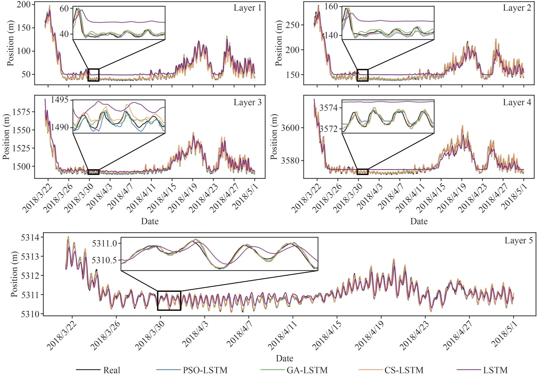
Fig.15 Comparison of predicted values among LSTM models of M2

Fig.16 Comparison of predicted values among LSTM models of M3
Besides, we noticed that the level of performance of the three moorings has a slight discrepancy, where the effectiveness of M1 and M2 is better than that of M3.From the information obtained from Fig.1, we can evidently find out that the observation location of the M3 is on the trajectory of the Kuroshio Extension, where is the high-incidence area of the ocean dynamic process (Sasai et al., 2010; Ma et al.,2015).We consider that the high nonlinearity of disturbances should be in charge of the weaker stability of M3.Further speaking, there has a small disparity of performance between M1 and M2 which may be caused by the eddy that exists near the position of M2 or the different makes of the moorings or their different weights.4.2.4 Simulation efficiency
Due to the high time resolution of the mooringmeasurements, seeking the optimal hyper-parameters is time-consuming and the quick response of the predicting algorithm is significant in the practical application, especially in deep-sea observations.Therefore, the excogitation of efficient and timesaving optimization methods is of great importance.In this study, we calculate the mean time consumption and the convergence of the proposed optimization algorithms in selecting the optimal solution of the LSTM neural network.The mean time of the GA,PSO, and CS is 1 668.32 s, 1 904.95 s, and 1 144.57 s,respectively and the convergence curve can be seen in Fig.18.It can be seen that CS has a quick convergence and can lead to the least time consumption according to the comparison among the three algorithms, which is the most efficient optimization strategy.

Table 6 Comparison of accuracy and percentage improvements

Fig.17 Comparison of mean-RMSE, mean-MAE, and mean-R2 values of three optimization algorithms
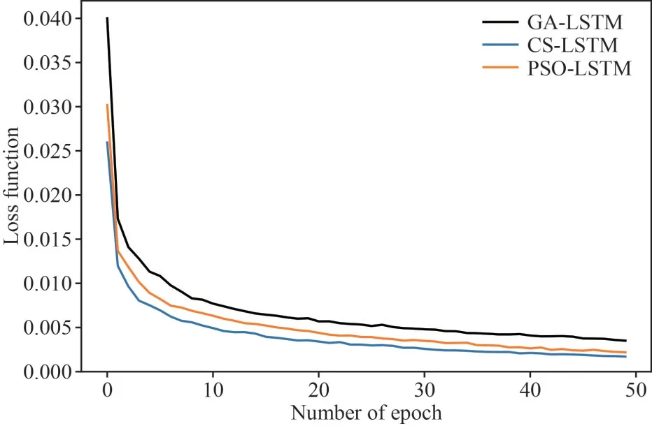
Fig.18 The comparison of convergence in the training processes on GA-LSTM, PSO-LSTM, and CS-LSTM
5 CONCLUSION
The ocean mooring array is an important component of the global observation system and the gold standard for obtaining successive in-suit profile measurements with high temporal and spatial resolution at a fixed location.However, the motion of the moorings is highly affected by the strong and variable ocean currents, which determine the quality of observations and the stability of the measurement formation of mooring arrays.Coupled with the high cost of the deployment and cooperative observation of mooring arrays make the design of the motion simulation model is necessary.In this paper, we propose a hybrid deep-learning simulation framework that is composed of LSTM neural network and optimization strategies to achieve mooring motion prediction under the high temporal resolution datasets.We integrate two main influence factors, namely the strength and direction of the ocean current and the position of the mooring into the simulation model to predict the motion trajectories of the mooring.Moreover, the cuckoo search optimization algorithm is used to tune the hyperparameters of the LSTM to improve the performance of the proposed model.The above workflow is automatic and fully datadriven, without any prior knowledge of the motion model.This characteristic improves the stability and generalization performance of the model together with higher flexibility for real-field applications.
We employ three mooring datasets to conduct experiments for the validation of the feasibility and effectiveness of the model.The results demonstrate that the proposed hybrid model has great improvements in performance and stability.Besides,we conduct explorations of predicting the longsequence motion of mooring; the results demonstrate that our proposed model can obtain good performance in the long-sequence motion prediction of moorings.Moreover, by the comparison with other optimization algorithms, including GA and PSO, the CS is much more efficient and has better convergence.
Furthermore, there is space for improvement to enrich the current study.Firstly, we need more datasets from different makes of moorings and different areas to evaluate the comprehensive performance of the model.Secondly, the study on the horizontal movement of moorings is still a gap; it is possible to investigate the horizontal movement based on the model in this paper.
6 DATA AVAILABILITY STATEMENT
The datasets generated during and/or analyzed during the current study are available from the corresponding author on reasonable request.
杂志排行
Journal of Oceanology and Limnology的其它文章
- A new decomposition model of sea level variability for the sea level anomaly time series prediction*
- Spatio-temporal dynamics of cyanobacterial abundance and toxicity in a Mediterranean hypereutrophic lake*
- Pharmacokinetics of fucoidan and low molecular weight fucoidan from Saccharina japonica after oral administration to mice*
- Diel, seasonal, and annual variations of fish assemblages in intertidal creeks of the Changjiang River estuary*
