A new decomposition model of sea level variability for the sea level anomaly time series prediction*

Qinting SUN, Jianhua WAN, Shanwei LIU,**, Jinghui JIANG,Yasir MUHAMMAD

1 College of Oceanography and Space Informatics, China University of Petroleum (East China), Qingdao 266580, China

2 Technology Innovation Center for Maritime Silk Road Marine Resources and Environment Networked Observation, Ministry of Natural Resources, Qingdao 266580, China

Abstract Rising sea level is of great significance to coastal societies; predicting sea level extent in coastal regions is critical.When carrying out predictions, the subsequences obtained using decomposition methods may exhibit a certain regularity and therefore can provide multidimensional information that can be used to improve prediction models.Traditional decomposition methods such as seasonal and trend decomposition using Loess (STL) focus mostly on the fluctuating trend of time series and ignore its impact on prediction.Methods in the signal decomposition domain, such as variational mode decomposition (VMD), have no physical significance.In response to the above problems, a new decomposition method for sea level anomaly time series prediction (DMSLAP) is proposed.With this method, the trend term in a time series can be isolated and the effects of abnormal sea level change behaviors can be attenuated.We decompose multiperiod characteristics using this method while maintaining the smoothness of the analyzed series.Satellite altimetry data from 1993 to 2020 are used in experiments conducted in the study area.The results are then compared with predictions obtained using existing decomposition methods such as the STL and VMD methods and time varying filtering based on empirical mode decomposition (TVF-EMD).The performance of DMSLAP combined with a prediction method resulted in optimal sea level anomaly (SLA) predictions, with a minimum root mean square error(RMSE) of 1.40 cm and a maximum determination coefficient (R2) of 0.93 during 2020.The DMSLAP method was more accurate when predicting 1-year data and 3-year data.The TVF-EMD and DMSLAP methods had comparable accuracies, and the periodic term decomposed by the DMSLAP method was more in line with the actual law than that derived using the TVF-EMD method.Thus, DMSLAP can decompose SLA time series better than existing methods and is an effective tool for obtaining short-term SLA prediction.

Keyword: time series decomposition; satellite altimetry; China Sea and its vicinity; sea level change

1 INTRODUCTION

Sea level is rising due to climate change (Church et al., 2013; Oppenheimer et al., 2019).This rise is expected to continue over the next few decades to hundreds of years and will have far-reaching effects on coastal areas (Wong et al., 2014).In low-lying areas, flooding and coastal erosion result from sea level rise; these processes can reduce land area and force coastal populations to migrate (Mimura,2013).In addition, sea level rise can increase water and soil salinization in coastal areas.Salinization impacts coastal agriculture, aquaculture, ecosystems and the supply of freshwater for domestic and commercial uses (Dasgupta et al., 2017).Since China began its economic reform in 1978, the growing national economy has become increasingly concentrated in coastal areas (Kanbur and Zhang,2005; Holz, 2008; Chen and Groenewold, 2010).These coastal areas have become economic zones with the highest economic densities, the strongest comprehensive strengths and the largest strategic support networks in China (He et al., 2014).According to the Statistical Communique of the People’s Republic of China on the 2020 Sea Level,sea level change exhibits a fluctuating upwards trend.From 1980 to 2020, the coastal level rise rate recorded in China was 3.4 mm/a, higher than the global average measured during the same period (Department of Marine Early Warning and Monitoring, 2021).Compared to traditional measurement methods,satellite altimetry technologies can obtain continuous sea surface height data and better analyze long-timeseries sea level changes over a wide range of sea areas.Currently, many types of high-temporalresolution and high-spatial-resolution satellite altimeter data are available, and these data are widely used to study sea level variations in vast sea areas and in other applications related to marine science (Cazenave et al., 2018).Based on satellite altimetry data,regular sea level change patterns can be studied in the China Sea and its vicinity.Thus, these data help the government respond promptly to the impacts of sea level rise in coastal areas.

Sea surface height data are often large-scale and nonlinear, and it is difficult to achieve high prediction accuracies with these data when using a single model.Rather, sea level can be better predicted by analyzing sea level trends and cycles.The index value influencing factors of sea level anomaly (SLA) time series can be divided into four categories: trend changes, seasonal changes, periodic changes, and random changes (Moosa, 1996).Longterm trend changes refer to the general continuous development and change trends of a time series over a long period (Jebb et al., 2015).Seasonal changes refer to obvious cyclical variations in time series caused by seasonal changes.Although the basic pattern of these changes is fixed, the magnitudes of the seasonal effects may change among different periods.Seasonal effects can also be embedded in overall trends (Geremew and Gourio, 2018).Therefore, the trend terms considered in this paper include the long-term trend changes and seasonal changes.Periodic changes involve fluctuations in time series over a period of several years.Random changes in a time series refer to nonperiodic or irregular trend changes caused by temporary or accidental factors (Hyndman and Athanasopoulos,2021).Many methods have been established for predicting sea level, including support vector machines (das Chagas Moura et al., 2010), artificial neural networks (Imani et al., 2013), extreme learning machines and relevance vector machines(Imani et al., 2018).Among existing methods, the seasonal autoregressive integrated moving average(SARIMA) is an extension of the autoregressive integrated moving average (ARIMA) model (Box and Jenkins, 1976) developed by Box and Jenkins(Tseng et al., 2002).SARIMA considers both periodicity and seasonal factors in a time series, and has a high prediction accuracy (Mao et al., 2018).Some time, long and short time memory (LSTM)networks can solve the gradient disappearance problem and have a good fitting effect on long time series data with poor regularity (Xiao et al., 2019).It is necessary to consider the characteristics of the analyzed time series when processing SLA time series, and multiple prediction models can be combined to improve the short-term sea level prediction accuracy.Therefore, the subsequences obtained by decomposing SLA time series exhibit a certain regularity and can provide multidimensional information that can be used by prediction models to achieve an improved prediction effect.

When conducting time series prediction, some scholars have considered using the signal decomposition method to decompose and process the time series data.An empirical mode decomposition (EMD)method, that can adaptively decompose signals into intrinsic mode functions (IMFs) and residual terms,was proposed by Huang et al.(1998).However, the EMD method has some problems; for example, the signal breakpoint is not necessarily the extreme point, so endpoint effects and modal aliasing problems can arise.Some time series decomposition algorithms depend on local data to obtain decomposition results, such as seasonal and trend decomposition using Loess (STL) (Cleveland et al.,1990) and X-13ARIMA seasonal adjustmenttime series (X-13ARIMA-SEATS) (Dagum and Bianconcini, 2016); among these algorithms, STL is the most classic.STL uses locally weighted regression and smoothing (Loess) steps (Cleveland, 1979) as a smoothing device to decompose a time series into a trend term, periodic term, and irregular residual term (Cleveland et al., 1990).STL can fit time series trends well, but trend changes can fluctuate due to the influence of random factors, and the existence of these fluctuations can affect the prediction accuracy.In addition, STL can decompose only one periodic subsequence and is not applicable to the decomposition of multiperiod time series.At times,series decomposition algorithms rely on all the available data and obtain each subsequence through a data value correlation decomposition at each incremental time point; these methods include singular spectrum analysis (SSA) (Broomhead and King, 1986), and variational mode decomposition(VMD) (Dragomiretskiy and Zosso, 2014).Since its development, SSA has been widely used in time series processing tasks because it can perform the stable functions of recognizing and enhancing periodic signals; however, this method suffers from overfitting issue (Elsner and Tsonis, 1996; Hassani,2007).VMD has a good effect on nonlinear signals,and the IMFs obtained by it are close to their corresponding center frequencies.The greatest limitations of VMD are boundary effects and bursty signals (Chouksey and Jha, 2021).Recently, Song and Chen (2021) compared five decomposition methods and found that time varying filtering based on empirical mode decomposition (TVF-EMD) method can improve the prediction accuracy.The subsequences obtained from TVF-EMD are relatively stable.The biggest disadvantage of TVF-EMD in the process of decomposing time series is that there is no specific physical explanation for the decomposed subsequences.

The main methods used to measure trend changes include regression analysis methods (Visser and Molenaar, 1995), moving average methods(Hansun, 2013), and envelope curve technique(Johnson et al., 2011).Regression analysis methods can roughly fit the growth trend of the time series and accurately predict the growth rate.The moving average methods can reflect the real fluctuating trends of the time series with random factors, and the existence of these fluctuations can affect the prediction accuracy.In the study of time series change, the envelope curve technique is to obtain the trend change by calculating the local maximum and local minimum of the time series and connecting and averaging them.However, the trend term obtained by this method is also affected by outliers.If the time series obtained by the envelope curve technique is smoothed, the influence of abnormal changes in a period of time can be better alleviated.In this paper, the trend term of the SLA time series is obtained by combining the envelope curve technique with Lowess smoothing (Cleveland,1979).The autoregressive integrated moving average (ARIMA) model (Box and Jenkins, 1976),multivariate model (King et al., 1991), and singular spectrum analysis (SSA) (Chen et al., 2013) are common methods used to extract period terms from time series after the trend term is removed.The advantage of the ARIMA model is that the model is very simple, only endogenous variables are required and no other exogenous variables are needed.The disadvantage is that the time series or series after differentiation is required to be stable.When decomposed using multivariate model and SSA, the periodic terms can exhibit certain tendencies or irregular fluctuation phenomena.The periodic terms with regular changes are obtained according to the period, and SLA time series predictions are carried out to avoid affecting abnormal values.In order to make the obtained period items more regular and predictable, the combination of moving average and Lowess smoothing methods are used to process the series composed of the same position in different periods.

To accommodate the temporal characteristics of the analyzed SLA time series, we proposed a new time series decomposition method for sea level anomaly time series prediction (DMSLAP).The DMSLAP was compared with the existing STL,VMD, and TVF-EMD decomposition models over the China Sea and its vicinity.Then, the SLA prediction accuracies obtained with the various methods were compared by combining different decomposition and prediction models.Finally, the DMSLAP method was used to compare the influence of different time scales on the SLA time series prediction.

This paper is organized as follows.In Section 2,three existing time series decomposition methods are described, and the proposed time series decomposition method is introduced.In Section 3,the experiments and the results were analyzed.The results and future research are discussed in Section 4.

2 METHOD OF TIME SERIES DECOMPOSITION

2.1 Existing decomposition method

In this section, two typical time series decomposition methods, namely, the STL and VMD methods, and a new method called TVF-EMD are introduced.These results obtained when conducting experiments on SLA time series datasets using these methods are then compared.

STL is a method used to decompose a time series into three parts: the trend subsequence, seasonal subsequence, and remainder subsequence.The STL is not affected by outliers in the data, and can estimate trend and periodic terms robustly (Cleveland et al., 1990).

The STL process consists of two loops, an inner loop nested within an outer loop.Within each inner loop, both the seasonal and trend subsequences are updated.The weight of each outer loop can be calculated using the results of the inner loop.The weight of the outer loop is then used in the next inner loop (Cleveland et al., 1990).The STL requires only 2 inputs, one is the time series to be decomposed, and the other is the period of the time series.The period entered is 12 in this experiment.

VMD is an adaptive nonrecursive decomposition method proposed by Dragomiretskiy and Zosso(2014), and this method decomposes signals into a sum of finite IMFs.VMD is used in crude oil prediction and image processing tasks and has shown superiority among existing decomposition methods (E et al., 2017; Chouksey and Jha, 2021).VMD requires a total of 7 input variables, expressed as VMD (s,alpha,tau,K,DC,i,tol).In order to satisfy the requirement that the SLA time series subsequences obtained using VMD are the trend term, periodic term, and residual term, the number of decomposition levelsKin the input parameters is set to 3.The other parameters are set as follows:sis the time series to be decomposed; the balancing parameter of the data-fidelity constraintalphais optimized by the genetic mutation particle swarm optimization algorithm, which is set to 2 000 in this paper; the update step sizetauis determined using the residual index indicator, which is set to 0 in this paper; true if the first mode is put and kept atDC, it is generally set to 0; the parameteridetermines the initial value of the center frequencyw, which is set to 2 in this paper; tolerance of convergence criteriontol, typically is approximately 1e-6 (Dragomiretskiy and Zosso, 2014).

TVF-EMD is an improved EMD model that uses time-varying filtering in the sifting process to solve the modal mixing problem and maintain timevarying characteristics.The TVF-EMD process consists of a total of three main steps: (1) estimate the local cut-off frequency; (2) construct a timevarying filter to obtain the local mean function and calculate the criterion value; and (3) judge whether the residual signal satisfies the stop criterion.The specific parameter selection process can be found in the cited literature (Li et al., 2017).The TVF-EMD performs an adaptive design of the local cutoff frequency by making full use of the instantaneous amplitude and frequency information, and each parameter is adaptively selected.Based on this, we only need to input the time series when decomposing.

2.2 Decomposition method for sea level anomaly time series prediction

According to the temporal characteristics of SLA time series, a new decomposition method for the SLA time series prediction is proposed, named decomposition method for sea level anomaly time series prediction (DMSLAP).In the proposed method, the trend term of the SLA time series is obtained by combining the envelope curve technique with Lowess smoothing, which can better alleviate the influence of abnormal changes over a period of time.In order to make the obtained period items more regular and predictable, the combination of moving average and Lowess smoothing methods are used to process the series composed of the same position in different periods.A flow chart of the DMSLAP process is shown in Fig.1.

The detailed steps for decomposing the SLA forPmonths are described below.

(1) According to the SLA time series sla(t),t=1,2, …,T, the average values of the upper and lower envelopes are obtained.The envelopes are determined using spline interpolation over local maxima separated by at least.The envelopes are determined using spline interpolation over local maxima separated by at leastnp(npis half the period of the time series)samples.Then, the mean value is used for Lowess smoothing to obtain the trend term slatrend(t) of the sea level anomaly time series.The window length wl is calculated for smoothing based on genetic algorithm (Ataee et al., 2007).The formulas used to calculate the trend term slatrend(t) at pointtare as follows:wheretkis thekthclosest point tot,k=1,2, …,wl;slamean(t) is the average value of the upper and lower envelopes.Bis a matrix of 1 and pointstk, which is used for matrix calculation.Wtis the diagonal matrix of weights.Kis the weight using the Epanechnikov quadratic kernel.Dis the Epanechnikov quadratic kernel.Yis all the slamean(tk) series in the windows with length wl centered at pointt.The schematic diagram of trend term slatrend(t) is shown in Fig.2.

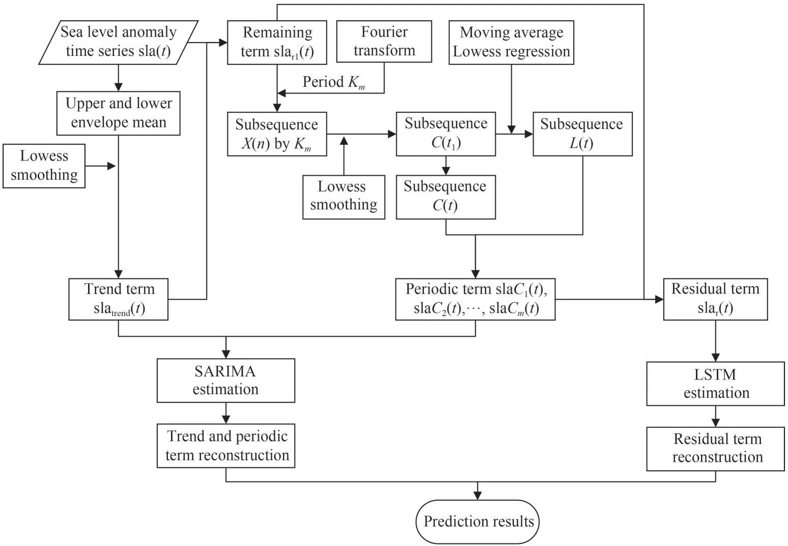
Fig.1 Flowchart of the decomposition method used in this study

The black dotted line in Fig.2 is the SLA time series sla(t).The blue curves in Fig.2 show the upper and lower envelopes of the SLA time series sla(t).The green line shows the average value of the upper and lower envelopes.The red line is the trend term slatrend(t).The trend term can reflect the series change trend and extract rules other than abnormal changes more accurately during the prediction process.

Fig.2 The trend term obtained from the schematic diagram

(2) The trend term slatrend(t) is subtracted from the sea level anomaly time series sla(t) to obtain the first remaining term slar1(t).Then, the period of the SLA time series is obtained by using Fourier transform (Goldblum et al., 1988).The number of periods ism, and the period isKm,m=1, 2, ….

(3) Using the first remaining term slar1(t)obtained in step (2), the periodic terms slaCm(t),m=1, 2, … of thePmonth SLA time series are calculated.

The specific process by which the periodic terms slaC1(t), slaC2(t), …, slaCm(t),m=1, 2, … are calculated according to the corresponding periodKmobtained in step (2) and are explained as follows:

Step 1: the first remaining term slar1(t) is grouped according to the periodKm, and each group of sample points derived at the same position constitutes subsequence setX(n)={slar1(n), slar1(n+Km), …, slar1(n+P–Km)}, whereKmis the period andn=1, 2, …,Km.

Step 2: lowess smoothing is used to perform a regression step for each subsequenceX(n), and the result is sequence setC(t1); then, each subsequence is extended forward and backwards forKmmonths to obtain the time seriesC(t2), wheret2=-Km+1, …,T+Km;T=P/Km.

Step 3: low-pass filtering of smoothed cyclesubseries is implemented.Moving averages are performed with window lengthsKm,Kmand 3 on the time seriesC(t2) in turn; then, the Lowess regression is performed to obtain the time seriesL(t),t=1, 2, …,T;T=P/Km.L(t) is equivalent to a low-throughput ofX(n).The periodic subsequence,C(t)=C(t1)–L(t),t=1, 2, …,T, is obtained by using time seriesC(t1) and time seriesL(t) (Cleveland et al., 1990).

Step 4: restore subsequence setC(t) to the periodic term slaCm(t) of lengthP.The schematic diagram of steps 1–4 is shown in Fig.3.

(4) By subtracting the trend term slatrend(t) and the periodic terms slaCm(t),m=1, 2, …, from the SLA time series sla(t) (1), the residual term slar(t) can be obtained.

3 EXPERIMENT AND ANALYSIS

In this paper, two experiments were conducted to verify the effectiveness of DMSLAP.First, a comparative experiment between DMSLAP and typical decomposition methods was performed.The DMSLAP, STL, and VMD decomposition methods were used to analyze the decomposition effect and completeness of each decomposition method.Then,the influence of the DMSLAP method on the SLA time series prediction effect is assessed on different timescales.When evaluating the prediction outcomes,we consider the mean, root mean square error(RMSE) and correlation coefficient (R2) as metrics.

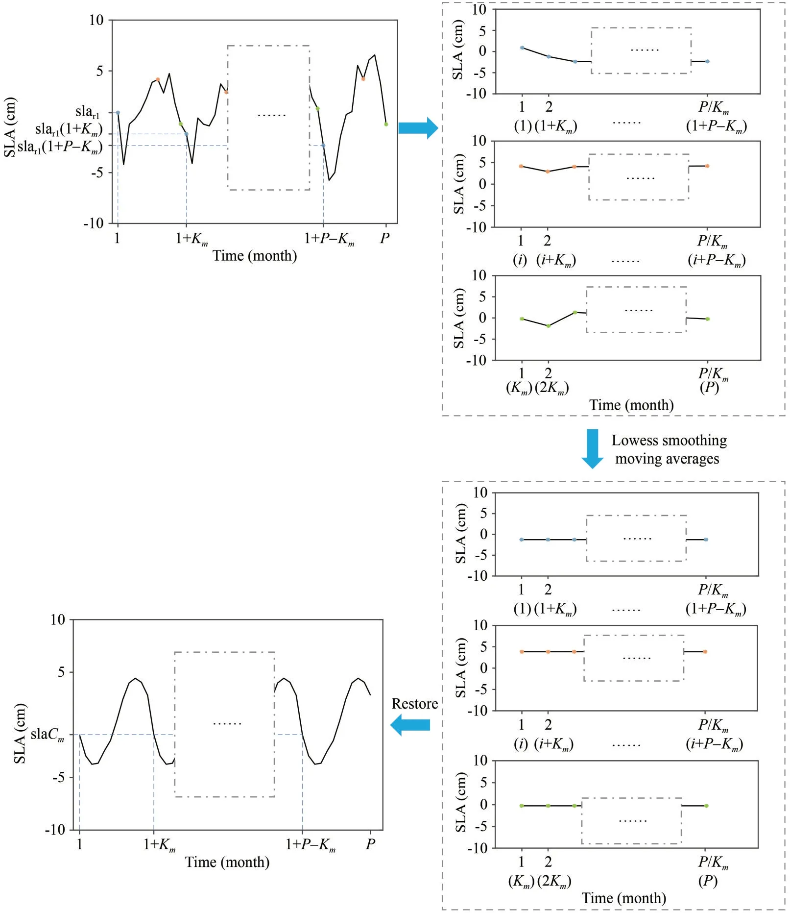
Fig.3 The schematic diagram of the periodic terms are obtained

3.1 Sea level anomalies data

The TOPEX/Poseidon (T/P), Jason-1, Jason-2,and Jason-3 satellite altimetry data recorded from 1993 to 2020 were used in this article.The study area spans from 105°E to 135°E and from 0° to 45°N,as shown in Fig.4.The reference sea level data used in this article is the mean sea surface-Centre National d’Etudes Spatiales-Collecte Localisation Satellites 15 (MSS_CNES_CLS15).This dataset is universally acknowledged as a high-accuracy global sea level model.The data used herein included geophysical data records (GDRs) from TP series satellite altimeters before the orbit change; these records were produced by CLS and distributed by Archiving, Validation and Interpretation of Satellite Oceanographic (Aviso+), with support from Centre National d’Etudes Spatiales (CNES) (https://www.aviso.altimetry.fr/).The timespan and cycles in the data recorded by each altimeter are provided in Table 1.

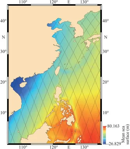
Fig.4 The research area and the tracks of satellites (black points) and the MSS_CNES_CLS15 model coverage range

Table 1 Satellite data used to establish SLA time series

First, the GDR data were divided by month.Next, the GDR datapoints associated with land flags and ice flags were removed.According to the handbooks (Blanc et al., 1996; Bronner et al.,2016; Dumont et al., 2017; Bignalet-cazalet et al.,2021) provided by CNES, data that did not meet the filtering criteria were also removed.Then, the sea surface heights were obtained through collinear and crossover adjustment processing steps (Jiang et al., 2002).The along-track SLAs were then obtained by subtracting the MSS_CNES_CLS15 reference sea level model from the derived sea surface heights.In the research area,monthly SLA data were obtained by the along-track SLA latitude-weighting method.The T/P data were used as a benchmark in this work to apply a system bias correction to the Jason-1, Jason-2, and Jason-3 SLA data.Finally, the monthly SLA data were corrected based on the biases among the four satellites in their tandem stages, as calculated by Wan et al.(2018).The time series of the SLAs discussed and analyzed are shown in Fig.5.

Figure 5 shows the 1993–2020 SLA time series derived after the processing steps.The sea level in the study area presents an overall rising trend,exhibiting an annual growth rate of 4.31 mm/a from 1993 to 2020.This growth rate is higher than the global annual sea level growth rate of 3.43 mm/a from 1993 to 2020 provided by the Aviso website (https://www.aviso.altimetry.fr/en/data/products/oc/ean-indicators-products/meansea-level/products-and-images-selection-within-saralold.html).The sea level rises and falls alternately and exhibits an obvious periodic change law.The sea level mainly decreases in spring and winter and gradually increases after reaching its minimum value in winter or spring.

Fig.5 SLA time series spanning 1993–2020

3.2 Decomposition of SLA time series

After processing, the SLA time series exhibits an obvious tendency and periodicity.The main purpose of the decomposition method is to decompose the temporal characteristics in a time series before further analyses or predictions are carried out.DMSLAP aims to decompose temporal characteristics for use in SLA time series predictions.This method not only ensures that temporal characteristics are represented but also reduces the influence of abnormal sea surface height changes on the accuracy of the prediction results.The effects of the DMSLAP, STL,VMD, and TVF-EMD methods on the decomposition process and results were further analyzed.

3.2.1 Time series feature extraction

The DMSLAP method decomposed a SLA time series into three parts: the trend term, periodic terms and residual term.In this paper, the DMSLAP method was used to calculate all local maxima and minima in the processed SLA time series.Then,based on the local maximum and minimum values,upper and lower envelopes were generated by cubic spline interpolation, and the mean values of the upper and lower envelopes were obtained.In addition,the trend term of the SLA time series was obtained by applying Lowess smoothing to the mean values,and the subsequence results are shown in Fig.6a.Then, the STL, VMD, and TVF-EMD methods were used to decompose the SLA time series, and the trend terms shown in Fig.6b, c, & d were obtained.

As seen from Fig.6, the sea level in the study area presented an overall fluctuating trend, and the derived trend terms could better reflect the fluctuation characteristics of the SLA time series when the four time series decomposition methods listed above were used.Among these four methods,the trend term obtained using the STL method can best reflect the real sea level change trend, and the significant rises and declines in sea level caused by El Niño and other climate phenomena are also reflected well.The trend terms obtained by the VMD and TVF-EMD methods are relatively similar,and both methods excessively smooth out details.Compared to the trend term obtained using the STL method, DMSLAP smoothed out the special change values, thus regularizing trend change.The trend terms decomposed by the VMD and DMSLAP methods can extract rules other than abnormal changes more accurately during the prediction process.

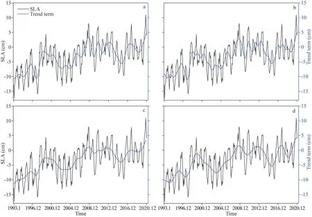
Fig.6 The decomposition results of the trend term obtained using different methods

After the trend term was obtained, in the DMSLAP method, the trend term subsequence was subtracted from the original SLA time series to obtain the first remaining term.The periods obtained by the Fourier transform are 12 and 30 months for the SLA time series, and the 100 periods such as 18 and 16 months are weak and can be ignored.The first remaining terms were sequentially divided into 12 months and 30 months in length, and each group of sample points derived at the same position constitutes a subsequence set.Then Lowess smoothing and low-pass filtering were performed on each subsequence.Finally, the periodic term was extracted from by restoring subsequence set.The resulting periodic term subsequences are shown by the blue curves in Fig.7a.The periodic term subsequence results obtained by the STL,VMD, and TVF-EMD methods are shown as blue curves in Fig.7b, c, & d, respectively.

The blue curves in Fig.7 show that some differences exist among the periodic terms obtained using the four methods.The periodic terms obtained using the VMD and TVF-EMD methods exhibit certain volatile characteristics, including periodic changes in some special cases.The periodic terms obtained by DMSLAP and STL are smoother than those obtained by VMD and are not affected by abnormal data behaviors.The STL method can decompose only one periodic sequence.DMSLAP considers the temporal characteristics of SLA time series, and the number of resulting decomposed periodic term subsequences are uncertain.Thus, the corresponding periodic subsequences can be calculated.

After obtaining the periodic term subsequence,the DMSLAP method subtracted the trend term subsequence and periodic term subsequence from the original SLA time series to obtain the residual term.The full results of the decomposition processes performed with the DMSLAP, STL,VMD, and TVF-EMD methods are shown as green curves in Fig.7a, b, c, & d, respectively.

We can see from the green curves in Fig.7 that most of the residual terms obtained using the four methods are within the range of -5 cm to 5 cm, indicating that these four methods can effectively decompose the SLA time series.Obvious differences can be observed among the results obtained with the four decomposition methods.VMD outputs other subsequences in addition to the trend term, periodic term, and residual term, and the total number of output subsequences is dependent on the inputs.The decomposition results obtained by the VMD and TVF-EMD methods are relatively similar, and the corresponding residual terms vary greatly and are difficult to predict.DMSLAP can decompose the data corresponding to the main period and other periods, and the main period results are similar to those obtained for the period decomposed by STL.

3.2.2 Time series decomposition similarity

In this work, cosine similarity was used to evaluate the similarity of two vectors by calculating the cosine value of the angle between them (Zhou and Leydesdorff, 2016).Equation 2 was used to calculate the cosine similarity and can be expressed as follows:

wherexandyare the original time series and the results after decomposition and the removal of the remaining subsequences, respectively, andTis the total amount of time covered by the analyzed data.

The similarities between the original SLA time series and the temporal subsequences decomposed by the four methods were calculated, and the results obtained are shown in Table 2.

Table 2 shows that the similarities between the results obtained using the four decomposition methods and the original series are high, and all similarity values are above 0.9.Thus, all four methods can decompose the time series well.The decomposition result obtained using the STL method best reflected the real sea level changes.This method had the highest degree of decomposition completeness compared to the other three analyzed methods.The cosine similarity of the DMSLAP result was slightly lower than that of the STL result.

3.3 Sea level anomaly time series prediction

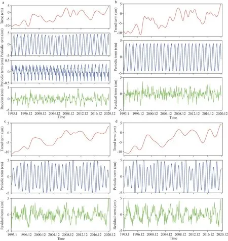
Fig.7 Time series decomposition using different methods

Table 2 Cosine similarities between the SLA time series and decomposition results

With regard to the decomposed SLA time series derived using the four methods, the combined SARIMA+LSTM method (Sun et al., 2020) was used to make predictions, and the predicted results were then analyzed.In this experiment, the data recorded from 1993 to 2019 were selected as the training set, and the data recorded in 2020 were selected as the verification set.Then, SARIMA was used to predict the trend terms and periodic terms, and LSTM was used to predict the residual terms.Finally, the prediction results were obtained by jointly predicting of the decomposed time series, and the results are shown in Fig.8 and Table 3.

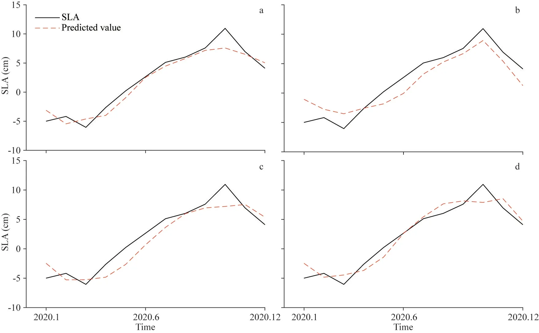
Fig.8 SLA time series prediction results using different methods

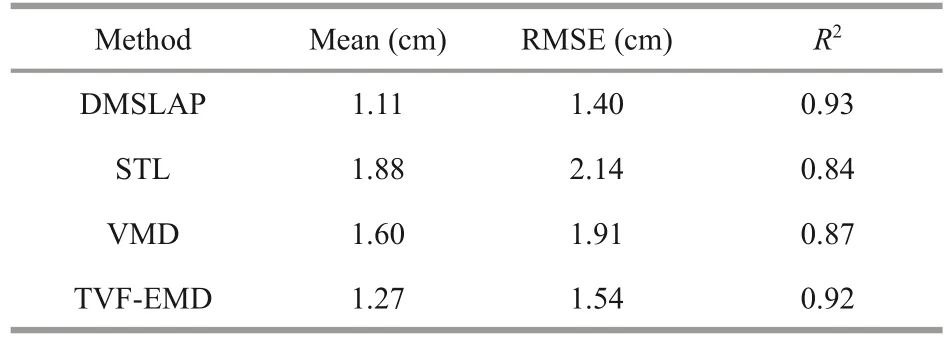
Table 3 SLA prediction results in 2020

As shown in Fig.8, the sea level change expected in the next year can be predicted to a certain extent by using the four methods analyzed in this work.Among these methods, the periodic term decomposed using the STL method was greatly affected by abnormal behavior, which further affected the periodic term prediction ability.The prediction effects of DMSLAP and TVF-EMD were equivalent.Table 3 also shows that among the four analyzed methods, the minimum RMSE value obtained by DMSLAP and the combined prediction model was 1.40 cm, and theR2value reached 0.93.The STL method provided the worst predictions, with an RMSE of 2.14 cm.The DMSLAP method was thus more conducive for SLA time series predictions than the STL method.Therefore, when conducting SLA time series predictions, in addition to the selection of the prediction method, which is very important, the selection of the time series decomposition method is also critical.During the decomposition stage, only by breaking down the regular components to the greatest possible extent can we obtain better predictions of the future conditions.

The DMSLAP decomposition effect was better than the effects of the other methods when predicting one-year SLA time series.We considered the influence of different time scales on the different decomposition methods analyzed.The DMSLAP,STL, VMD, and TVF-EMD methods were used to predict SLA values during 2020, 2019–2020, and 2018–2020 based on SLA time series data records of 1993–2019, 1993–2018, and 1993–2017, respectively.The sea level prediction results obtained in these different time periods using the four methods listed above are shown in Table 4.

As we can see from Table 4, the effect of DMSLAP was greatly affected by the analyzed time scale.On different prediction time scales, the prediction effect exhibits certain differences.Looking only at the DMSLAP prediction results, we can see that the longer the prediction time is, the worse the prediction accuracy is when using thesame decomposition and prediction methods.As seen from Table 4, the prediction accuracies of the four decomposition methods generally decrease when the prediction time length increases.The DMSLAP method has the highest accuracy when forecasting only 1-year data, the TVF-EMD method has the highest accuracy when predicting 2-year data, and the DMSLAP method has the highest accuracy when predicting 3-year data.Among these results, the RMSEs of the STL and VMD methods are concentrated at approximately 2 cm, and these values are excessively large among the three groups of experiments; thus, these two methods are not suitable for short- or medium-term SLA time series predictions.The TVF-EMD method performs slightly worse than the DMSLAP method when predicting 1-year data and is slightly more accurate than DMSLAP when predicting 2-year data; conversely, the DMSLAP method is more accurate when predicting 3-year data.Overall, the TVF-EMD and DMSLAP methods have comparable accuracies.However, the periodic term decomposed by the DMSLAP method is more in line with the actual law than that derived using the TVF-EMD method.When DMSLAP is combined with the prediction model, the short- and medium-term time series prediction accuracies are increased.Therefore, DMSLAP can play a substantial role in short-term sea level anomaly predictions.

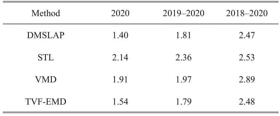
Table 4 The RMSEs derived after SLA time series predictions (unit: cm)

4 CONCLUSION

According to the temporal characteristics of SLA time series, we proposed a new decomposition method for predicting SLA time series in this paper.The purpose of the developed method is to improve the sea level change prediction accuracy, named DMSLAP(decomposition method for sea level anomaly time series prediction).This developed method and the existing STL, VMD, and TVF-EMD methods are used to decompose SLA time series.The comparison results of the decomposition experiments show that:

(1) from the decomposed trend items, it is found that the trend items obtained using the STL method can best reflect the real sea level change trend,which is more advantageous for analyzing the trend growth of sea level change directly.However, the VMD and DMSLAP methods can maintain the overall trend while removing the influence of abnormal data behaviors on the decomposed trend terms, which can better predict sea level changes.

(2) from the decomposed periodic terms, it is found that the periodic terms obtained using the VMD and TVF-EMD methods are unstable in some special cases.The periodic terms obtained using the DMSLAP and STL are smoother and unaffected by abnormal data behaviors.The DMSLAP can maintain the overall change characteristics while maintaining the smoothness of the time series,reducing the difficulty of SLA time series prediction.

Experimental studies on the SLA prediction were carried out in the China seas and its vicinity.The DMSLAP, STL, VMD, and TVF-EMD methods were designed to predict 1-, 2-, and 3-year SLA values.The DMSLAP method was more accurate when predicting 1-year data and 3-year data.TVFEMD and DMSLAP had comparable accuracies,and the periodic term decomposed by the DMSLAP method was more in line with the actual law than that derived using the TVF-EMD method.These results show that DMSLAP has a higher decomposition completeness and a better prediction effect than the other existing methods and is thus an effective tool for predicting short-term sea level changes.Although SLA time series are complex, the DMSLAP method can successfully decompose the corresponding trend and period terms when only temporal variables are considered.In future studies,we may consider the impacts of various prediction methods on decomposition methods analyzed herein, as multiple prediction methods were not evaluated in our current work.

5 DATA AVAILABILITY STATEMENT

Publicly available datasets were analyzed in this study.The satellites altimetry data can be found here: AVISO website (https://www.aviso.altimetry.fr/).

6 ACKNOWLEDGMENT

The authors also wish to thank the AVISO website of the French Space Center (CNES) for providing the satellite data.