Wind-speed forecasting model based on DBN-Elman combined with improved PSO-HHT

Wei Liu,Feifei Xue,Yansong Gao,Wumaier Tuerxun,,Jing Sun,Yi Hu,Hongliang Yuan

1.Northwest Engineering Corporation Limited,Xi’an 710000,P.R.China

2.College of Energy and Electrical Engineering,Hohai University,Nanjing 210098,P.R.China

Abstract: Random and fluctuating wind speeds make it difficult to stabilize the wind-power output,which complicates the execution of wind-farm control systems and increases the response frequency.In this study,a novel prediction model for ultrashort-term wind-speed prediction in wind farms is developed by combining a deep belief network,the Elman neural network,and the Hilbert-Huang transform modified using an improved particle swarm optimization algorithm.The experimental results show that the prediction results of the proposed deep neural network is better than that of shallow neural networks.Although the complexity of the model is high,the accuracy of wind-speed prediction and stability are also high.The proposed model effectively improves the accuracy of ultrashort-term wind-speed forecasting in wind farms.

Keywords: Wind-speed forecasting; DBN; Elman; HHT; Combined neural network

0 Introduction

Recently,the vigorous promotion of wind power has led to significant economic benefits; however,wind farms face several technical challenges [1].For example,the WT output is affected by the intermittency and randomness of wind.This hinders the integrated development of windpower systems [2] and can seriously impact the stability of grid-connected systems,impeding the scheduling and control of wind farms.Accurate and effective output power prediction is key to solving the aforementioned issues.The output power of a WT is a function of the wind speed,and accurate prediction of wind speed is the basis for wind-farm output-power prediction [3].Improving the accuracy of wind-speed forecasting is thus crucial for both wind-power and grid systems.Therefore,it is important to study the improvements in wind-speed prediction.Over the past few decades,several forecasting methods for wind speed and power have been proposed [4].Ultrashort-term wind speeds are typically encountered in wind-farm control,powerquality assessment,and mechanical-component design [5].The commonly used forecasting methods for ultrashortterm wind speeds include the Missing interpolation model for wind power data based on the improved complete ensemble empirical mode decomposition with adaptive noise (CEEMEAN) method and generative adversarial interpolation network model [6],spatial correlation method[7],and Support vector regression (SVR) [8].Currently,deep-learning methods such as convolutional neural networks (CNNs),deep belief networks (DBN),Recurrent neural networks (RNNs),and long short-term memory(LSTM) are used to predict the wind speed in wind farms [9].The nomenclatures are listed in Table A1.

The inherently strong turbulence and nonlinear velocity make wind-speed prediction difficult.The prediction accuracy of a single physical or statistical model often cannot meet the requirements of power-grid dispatch and wind-farm control.However,data preprocessing using signal-analysis methods can effectively improve the prediction performance.This study utilizes the Hilbert-Huang transform (HHT) to establish a signal-decomposition model,owing to its adaptability and suitability for nonlinear and nonstationary signal processing.However,in practical applications,the high-frequency components obtained through the empirical mode decomposition (EMD) in the HHT process generally exhibit with more severe oscillations.This significantly affects the overall forecasting accuracy,imposing greater requirements on the forecasting model.Previous research on HHT-based forecasting had neglected the effects of individual intrinsic mode functions(IMFs) with unique frequencies on the forecasting outcomes.Rather,they directly superimposed the forecasting outcomes of all components [10].To improve the performance of the original HHT-combined forecasting model,this study proposes an improved particle swarm optimization(IPSO) algorithm to analyze the weight coefficient of each IMF component.This approach effectively enhances the accuracy of the forecasting model.Artificial intelligence models such as Artificial neural network ANN are widely used for date forecasting because of their ability to learn from historical data.Currently,ANNs usually feature a single-hidden-layer network structure and therefore,fail to achieve the desired accuracy.For example,the DBN toplevel BP algorithm lacks memory functionality for training samples and is prone to a local optimum.

To solve these issues,we establish a combined windspeed forecasting model that utilizes both the DBN and Elman neural network.The proposed ultrashort-term windspeed forecasting model combines the DBN-Elman model with the improved Particle swarm optimization (PSO)-HHT algorithm,resulting in a highly accurate forecasting model.This new model further enhances the forecasting performance and offers promising results.

This study proposes two main innovations:

1) Replacement of the commonly used Back propagation(BP) algorithm in the DBN with the Elman neural network and establishment of the DBN-Elman combined wind-speed prediction model.This overcomes the disadvantages of the BP algorithm,such as the lack of memory functionality while training the samples and vulnerability to local optimal solutions.

2) Optimization and improvement of the HHT prediction performance using PSO.

The combination of these two innovations leads to the proposed DBN-Elman ultrashort-term wind-speed prediction model based on the IPSO-HHT,which not only optimizes the training performance but also enhances the overall prediction performance.

1 Methodology

1.1 DBN-Elman model

The DBN-Elman model is established by combining the DBN and Elman neural networks,taking advantage of the ability of deep learning to automatically learn the internal characteristics of the sample data.First,the windspeed training samples are linearly normalized.Then,the restricted Boltzmann machine (RBM) parameters are trained and updated using the contrast divergence (CD) algorithm.The samples obtained after feature extraction using the DBN are input to the Elman network.The Elman network parameters are updated using BP,by comparing the output value with the actual wind speed,until the stopping criterion is satisfied.This technique ensures that the model accurately represents the real-time variations in wind-speed readings.

For the regression problem,the top layer of the DBN generally uses the BP algorithm.The output when using BP as the top-layer algorithm in the DBN can meet the requirements of accuracy; however,this method is associated with problems such as incomplete training,easy loss of features of previous trained samples,and difficulty in achieving global optimality.In this study,a novel high-level algorithm called the Elman neural network is used for wind-speed forecasting in wind farms.Unlike a regular feedforward network,the Elman network features an additional bearing layer similar to a delay operator,endowing it with memory functionality and enabling it to directly reflect the dynamic characteristics of the control system,with stronger computing ability and higher network stability.In this study,a DBN-Elman combined neural network is established,which combines the powerful data-feature-extraction performance of the DBN with the dynamic characteristic feedback functionality of the Elman network.The structure of the proposed DBN-Elman model is presented in Fig.1;v1,v2andh1,h2represent the visible and hidden layers of RBM1 and RBM2,respectively,and the number of hidden-layer nodes in RBM1 is the same as that in RBM2.

Fig.1 Structure of the DBN-Elman model

The training process for the DBN-Elman model involves two stages: unsupervised training for the DBN and supervised training for Elman.The unsupervised training of the DBN aims to mine the deep characteristics of data and obtain the training parameter values for the entire DBN.This is more efficient than supervised training and can thus improve the training efficiency of the DBNElman combined model.In the supervised training process for Elman,the parameters obtained from DBN learning are typically used to obtain the forward propagation results of the network,which are compared with the actual values for error calculation.Finally,the Elman parameters are reversely adjusted using the gradient-descent method to further optimize the effectiveness of the DBN-Elman model.The training procedure for the DBN-Elman model is presented in Fig.2.

Fig.2 Training procedure of the DBN-Elman model

1) Parameter initialization: Network parameters such as the number of network layers and nodes in each layer,rate of learning,weight,bias,and highest number of epochs are initialized after training and data preprocessing.

2) Training RBM1: The visible layerv1of RBM1 is the input layer of the entire network,whose number of nodes should be consistent with the input dimensions of the forecasting model.The parameters of RBM1 are trained and updated according to the CD algorithm,and are eventually determined after training.

3) Training RBM2:h1andh2are considered the visible and hidden layers,respectively,of RBM2.The RBM2 parameters are trained and updated according to the CD algorithm and are determined after training.The network training continues according to the above steps until all RBMs are trained.

4) Elman parameter adjustment: The training samples are input to the model according to the fixed forecasting input window and propagated from the bottom to the top,to the last hidden layer of the DBN.Subsequently,the samples after feature extraction by the DBN are input to the Elman network.In the final stage of our experiments,the output value of the Elman network is evaluated against the real wind speed.We then employ the widely used BP technique to modify the parameters until the predefined termination condition is satisfied.The stopping criteria are established to either achieve the target accuracy level of the objective function or adhere to the time limit for training and reach the highest number of iterations.The expression for the objective function is

whereSdenotes the number of output neurons,Yk(t) andyk(t) represent the desired and actual output of thek-thoutput neuron at the t-th iteration,respectively.

5) Thus,the DBN and Elman parameters are determined and the training of the DBN-Elman combined model is completed.

1.2 HHT

In 1998,Huang et al.introduced the HHT,which is an EMD technique [11] that is intuitive,efficient,adaptable,complete,reconfigurable,and easy to implement with excellent time-frequency convergence [12].HHT is very effective in processing nonstationary and nonlinear signals,and is well-suited for application in various fields such as engineering,geophysics,and biomedical research.The HHT is a combination of the Hilbert transform and EMD technique.EMD assumes that each IMF is independent of the other components in the decomposition.

This study applies the HHT approach to analyze the time series of wind speeds [13].The decomposition process is as follows.

1) The cubic-spline method is used to fit the highest and lowest points of the signalv(t),resulting in the formation of upper and lower envelopes of the original data sequence.

2) To obtain the difference signalh1(t),the mean value of the envelopem1(t) is calculated and subtracted from the original signalv(t).

3) Ifh1(t) meets the IMF conditions,markc1(t)=h1(t).Then,c1(t) is defined as the first component of the IMF; it is the most frequent component of the original sequence.Otherwise,h1(t) is regarded as a newv(t) and the EMD process is repeated multiple times (generally denoted byk) until the difference signalh1(t) satisfies the conditions of an IMF.

(4) To obtain the remaining components,a constantc1(t)is subtracted from the original signalv(t):

After applying the EMD method to a new raw data signalr1(t),the same steps are repeated to obtainnIMF components and one residual component.The results are expressed as follows.

Whenhi(t) is satisfied,the given termination condition will be satisfied,and the signal decomposition will be complete.The original time series can be expressed as

whereci(t) is the component representing the different time characteristic scales of the signal,whose scales range fromc1(t) tocn(t),representing a transition from the highto low-frequency components.rn(t) is the residual function showing the average overall pattern of the signal.In this study,the Cauchy-like convergence criterion proposed by Huang et al.serves as the component termination condition;that is,the standard deviation (SD) coefficient of the results of two consecutive IMF screening sequences is used as the evaluation standard [14],which is determined as

whereTrepresents the number of samples of the sequencehi(t),andαis a small preset value (0.1 in this paper).When SD is less than or equal toα,the filtering process is terminated.The Hilbert transform is the convolution of a temporal sequenceX(τ) with the function 1/t.

whereτis an integral variable,Tis the amount of displacement of function -1/τ,andPrepresents the Cauchy principal value.

According to the above definition,the complex conjugate analytical signal can be obtained fromX(t) andY(t) as

Equations (6) and (7) represent the characteristics of the localX(t),anda(t) andθ(t) represent the instant amplitude and phase,respectively,after the Hilbert transformation,and can be mathematically represented as

Then,the expression for instant frequency is:

However,for a simple signal,the instantaneous frequency is meaningful only when the signal satisfies the local symmetry of the zero-mean value.

The HHT is adept at handling nonlinear and nonstationary data because of its ability to decompose a signal determined by the local characteristics of the internal time scale [15].The data processing mainly includes two parts—decomposition of the data using EMD and analysis of the spectra of the several components obtained from the decomposition.Many researchers have focused on the advantages of HHT in signal analysis and have applied it to many different fields such as mechanical fault diagnosis,medical signal analysis,seismic signal processing,fluid mechanics,and language signal processing.

1.3 PSO algorithm and its improvement

Reducing redundancy: The Boid model,which can mimic the flocking behavior of birds,serves as the basis for PSO [16].In this algorithm,the behavior of each particle is affected by its surrounding individuals.The rules to be considered during the flight of each particle are as follows [17]:

1) Avoid collisions: Avoid collisions with nearby individuals.

2) Consistent speed: Fly at a speed consistent with the average speed of the nearby individuals.

3) Gather towards the center: Move towards the mean position of neighboring individuals.

The PSO algorithm is a parallel and random optimization algorithm that uses competition and cooperation among individuals to perform a global search.In the search space,a group of random particles is initialized to form a population.Each particle corresponds to a group of solutions.The particles complete the optimization by tracking two “extreme values.” The two types of “extreme values” are individual and global,namely,the optimal position searched for by the particles and the entire population [18].The easy operation,simple algorithm,low requirements of the optimized function,and fast convergence of the PSO algorithm make it suitable for application in various fields.This study applies PSO to establish a model for predicting wind-speed combinations.

The fundamental PSO algorithm updates the flight position and speed of each particle using the following method:

wherevid(t) andxid(t) represent thed-dimensional values of the velocity and position vector,respectively,of particleiat thet-th iteration;pidandpgdcorrespond to thed-dimensional values of positionpiandpg,the optimal solutionpis the most suited for both particleiand the population;c1andc2represent the acceleration factors; andrand1() andrand2() represent random functions that generate random numbers in [0,1].

Shi and Eberhart introduced inertia weights to the PSO algorithm,which improved the optimization process [19].The improved model,also known as the standard PSO model,can be expressed as

whereωrepresents the inertia weight.The fundamental PSO algorithm can be regarded as the standard PSO model forω=1.

With the predetermined inertia weightω,the current speed of the particles can vary with the number of iterations,owing to the influence of the historical velocity.The searchability of the PSO algorithm can be adjusted by changingω; therefore,ωis introduced to eliminate the dependence of the fundamental PSO algorithmVmax.IfVmaxis small,ωcan be increased to achieve a balance between local and global searches,which increases the number of iterations.At this time,Vmaxcan be considered a fixed value and onlyωis adjusted.The lesserωis,the frailer the global search capability will be.

Shi and Eberhart [20] proposed a linearly decreasing weight strategy to adjust the inertial weight as

whereωiniis the initial inertia weight,generally set as 0.9;ωendrepresents the inertia weight used during the final iterations of the algorithm,generally set as 0.4;Tmaxrepresents the total number of iterations; andtindicates the current iteration.

This study focuses on weight decline and proposes a nonlinear weight-declining strategy based on the linear weight-decline strategy adopted by Shi and Eberhart,which then provides the two specific implementation methods described below.

1) Implementation method 1

wheretis the current iteration number andωeis the lowest momentum weight,taken asωe=0.4.The variation inωat this point is shown in Fig.3.ωgreatly changes when the number of iterations is less than 10; however,it changes gently and generally stabilizes when the number of iterations is greater than 10.In general,the inertia weightωfirst changes rapidly and then slowly.

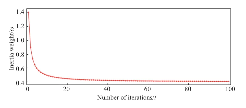
Fig.3 Change in inertia weight ω

2) Implementation method 2

wheretis the current iteration number,Tmaxis the highest iteration count,andωeis the limited minimum inertia weight,generally set as 0.4.The variation inωat this point,is shown in Fig.4,whenTmax=100.The figure shows thatωchanges slowly when the number of iterations is less than 20,whereas it demonstrates rapid changes when the number of iterations is greater than 20.In general,the inertia weightωchanges slowly in the beginning; later,it changes rapidly,with a relatively uniform amplitude,unlike implementation method 1.

Fig.4 Change of inertia weight ω

The IPSO algorithm’s modeling procedure is outlined below:

1) Population initialization: Initialize population sizenas 30.The particle dimensionDis consistent with the number of elements,which is 9,The acceleration constantsc1=c2=1.494.The highest iteration countTmax=100.Given the range and velocity limits of the weight coefficient,a random particle swarm is generated.

2) Determination of the fitness function: The optimal weight coefficients of the particle swarm are determined by evaluating its fitness function,by employing the Root mean square error (RMSE).

3) Evaluation of particle swarms: Calculate RMSE for every individual in the group,and compare it with the present RMSE value of the particle that has the optimal RMSE value; when the present RMSE value is smaller,the present location of the particle is considered optimal.Each particle’s current RMSE value is evaluated against the global extremum’s RMSE value,and the current optimal location of the population is determined as the coordinates of the particle with the smallest RMSE value.

4) Update the location and speed of the particles according to Equations (12) and (13).

The inertia weightωis renewed as:

whereTmaxrepresents the highest iteration count;tis the current iteration number.ωinirepresents the initial value for the inertia weight,which is set as 0.9;represents the inertia weight that pertains as the system advances towards the highest iteration count,which is set as 0.4; andωeis the limited minimum inertia weight,set as 0.4.

5) Upon reaching the highest number of iterations,denoted asTmax,the algorithm concludes its execution.

1.4 HHT method based on IPSO algorithm

The serious oscillation of high-frequency components detached from the EMD has a significant influence on the overall forecasting accuracy and imposes high requirements on the forecasting model.The existing research on HHTbased forecasting directly superimposes the forecasting results of all components [10],ignoring the effects of IMF components of different frequencies on the forecasting results.Therefore,in this investigation,an enhanced standard PSO algorithm is employed to study the weight coefficients of each IMF component,which effectively improves the capability of the original HHT combined forecasting model.

According to the HHT theory,the primary wind data are decomposed intonIMF components and one remaining component,represented by

whereci(t) represents thei-th IMF element of the wind-speed series andrn(t) represents the remaining element.Generally,the Hilbert transform is employed to perform a spectral analysis of the decomposed IMF components and establish forecasting models for thenIMF components and one residual component,according to their spectral characteristics,to predict the wind speed.The final forecasting result is determined as follows:

1) Before improving the HHT,the forecasting results of each component are directly superimposed to obtain

2) After the improvement of the HHT,the IPSO algorithm is employed to dynamically calculate the weight coefficients of every component,and finally superimpose the forecasting results of each component according to the weight coefficients as

2 DBN-Elman forecasting model based on IPSO-HHT

Because of the inherently strong randomness and turbulence of wind speed,this study establishes a combined forecasting model that relies on data preprocessing and weight allocation.This model preprocesses the wind-speed data using the HHT model and achieves weight distribution using an IPSO algorithm.First,the temporal sequence of wind speed is decomposed into a sequence of comparatively stable IMF components and a residual component,using the EMD method,which relies on data preprocessing via the HHT method.Then,the Hilbert transform is sequentially implemented for every individual element,and different DBN-Elman neural network models are established for forecasting according to their spectral characteristics.Finally,based on the forecasting results of each component,an algorithm is employed to compute the weight coefficient associated with each component.The final forecast windspeed is acquired by superimposing the weight coefficient by considering the projected results of each element.

Solving the weight coefficient of each component not only overcomes the inability of the fixed weight coefficient to accurately adapt to the varying time series of wind speed but also increases the flexibility and efficiency of the weight coefficient.In the actual forecasting process,the present wind-speed value remains uncertain; thus,the predicted wind-speed value is computed at the current time using the weight coefficients obtained previously.The detailed forecasting procedure is illustrated in Fig.5.

Fig.5 Flowchart of combined forecasting

The basic process is summarized below:

1) Decompose the time sequence of the wind speed using EMD.

2) Employ Hilbert Transform to the decomposed components in turn and establish different DBN-Elman neural network models for forecasting,according to the spectral characteristics of the components.

3) Establish an IPSO model.

4) Use the IPSO to calculate the weight coefficients of each component.

5) Obtain the ultimate wind-speed forecasting result by superimposing the forecasting results of each component according to the weight coefficient.

3 Experimental results and discussion

3.1 Data preprocessing

In this study,wind-speed time-series data were obtained from a WT of a wind farm in Jingbian,Shanxi,China.The actual wind-speed time series from August 22,2015,to September 4,2015,were selected as the experimental data.The temporal resolution of the data was set to one minute.After data collection and cleaning,7200 groups were used as experimental samples.Among them,the first 7140 groups were used as the training samples,and the remaining 60 groups were treated as the testing samples,as shown in Fig.6.Table 1 presents the statistics of the training and testing samples.

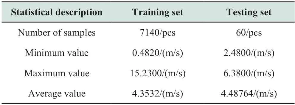
Table 1 Statistics of training and testing samples

Table 2 Training results of the structural parameters for different components corresponding to the DBN model

Fig.6 Wind-speed time-series data

Fig.6 illustrates the wind-speed time-series data,which are highly volatile and jagged.

Fig.7 shows the frequency distribution of the windspeed data.Table 1 and Fig.7 demonstrate that the wind speed is predominantly between 4.5 and 8.5 m/s,which is generally in the medium range of 1.93 to 12.77 m/s.In this study,the wind-speed data are found to follow a Weibull distribution,as evidenced by the two-parameter Weibull distribution curve shown in Fig.7.The shape factorkand scale factorcare 4.3633 and 7.3178,respectively.

Fig.7 Frequency distribution of wind-speed data

To address the nonlinear and volatile properties of wind-speed signals and facilitate their forecasting,the wind-speed data discussed in this study were decomposed and processed.Fig.8 shows the EMD outcomes for the initial data.As shown in the figure,these components are decomposed into nine IMF components and one remaining component.Fig.8 shows that the IMF components exhibit a sequential increase in their time-feature scales,from IMF1 to IMF8,concomitant with a shift in the frequency from high to low.

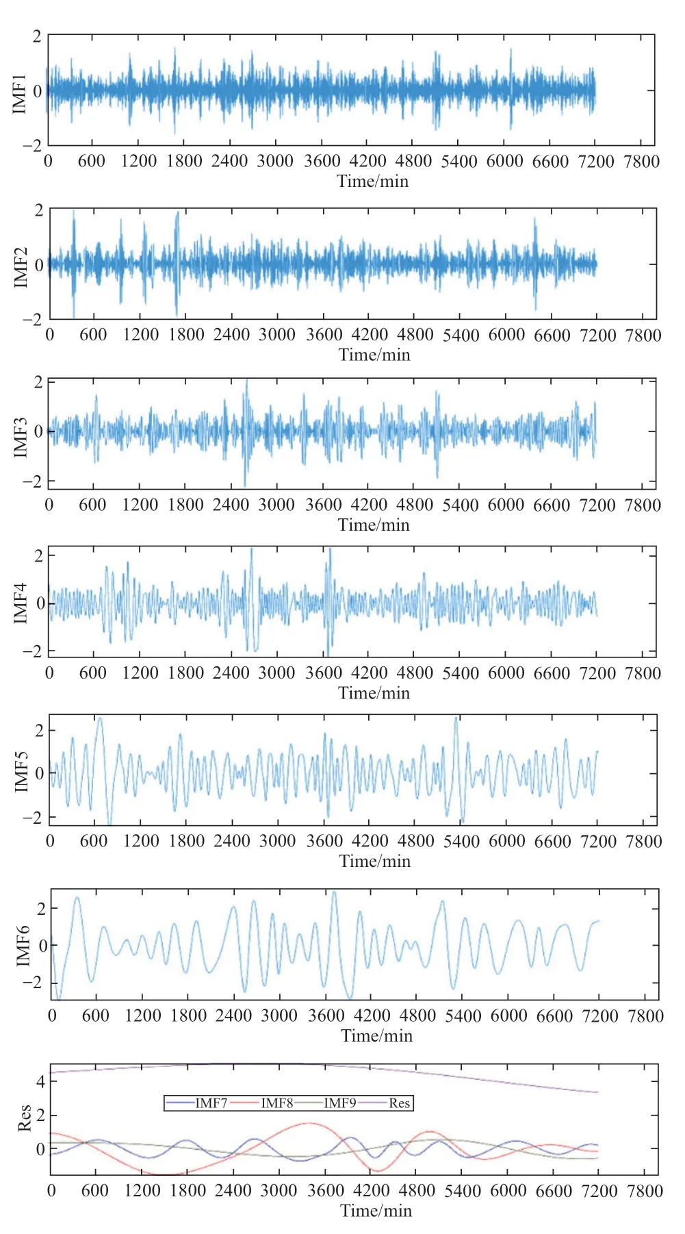
Fig.8 EMD decomposition results of raw wind-speed data

3.2 Parameter setting

The DBN and DBN-Elman models suitable for the different components were individually established.The training results for the structural parameters of the two Deep neural network (DNN) models corresponding to the different components are presented in Tables 2 and 3.

3.3 Predictive performance evaluation metrics

Merely visualizing the final forecasting results is not sufficient for understanding.Instead,they must be quantified to be more intuitive.

Hence,it is important to rationally opt for appraisal indicators pertaining to wind speed and power forecasting errors to judiciously assess the efficacy and pragmatic applicability of the proposed prognostic model.The present study employs evaluation measures including the RMSE,MAE,MAPE,andR2.Their expressions are as follows [21]:

wherexotrepresents the actual data at timet,represents the predicted data at timet,represents the average value,andNrepresents the total number of samples in thex(t)sequence.The RMSE reflects the statistical characteristics of the error,which is used to quantify the disparity between the observed and anticipated values,and delineate the extent of scatter within the specimen.Therefore,the more novel the RMSE,the smaller the deviation and higher the prediction accuracy will be.MAE,which denotes the arithmetic mean of the absolute deviation between the observed and estimated values,is a measure of the model performance and can be regarded as a linear combination of individual absolute errors,with all individual errors having the same weight.Therefore,the smaller the average error of the MAE prediction,the higher the overall prediction accuracy.The numerator part ofR2represents the sum of the difference between the squares of the real and predicted values,similar to the Mean squared error (MSE),and the denominator represents the sum of the difference between the squares of the real and mean values,similar to the variance,which can indicate the quality of the model fitting.Generally,the largerR2is,the better the model-fitting effect will be.

3.4 Experimental results and discussion

When calculating the final forecasting result,the combined forecasting method,which preprocesses the original data along with the HHT and model-decomposed components,frequently superimposes the anticipated outputs of each component without considering the influence of the component on the forecasting result.An enhanced PSO method is used to investigate the weight coefficients of each IMF component and the residual element.The final prediction results of the model are obtained based on the weight coefficients.

Fig.9 displays the forecasting effects of the Elman,LSTM,DBN,DBN-Elman,HHT-DBN,HHT-DBN-Elman,IPSO-HHT-DBN,and IPSO-HHT-DBN-Elman models.It is apparent from the illustration that the shallow Elman neural networks demonstrate poor forecasting effects and fail to respond to sudden changes in wind-speed data in realtime,with an obvious time lag; the deep neural networks of LSTM,DBN,and DBN-Elman exhibit better forecasting performance than the shallow neural networks; nevertheless,it is difficult to accurately forecast the sawtooth fluctuations in wind speed.The forecasting performances of the DBN and DBN-Elman models combined with HHT to pretreat the wind-speed data are significantly superior to that of the simple DBN and DBN-Elman networks,with a stronger ability to respond to sudden changes in wind-speed data;however,there is still room for improvement.The projected outcome of the DBN hybrid model combined with the enhanced PSO-HHT is depicted by the solid green line.The graph shows how the HHT decomposition prediction results for each component are obtained using the IPSO method.The overall forecasting results are produced by layering the data using a weight coefficient.The evaluation results of the aforementioned models are presented in Table 4.If the value of the paired t-test is less than or equal to 0.05,the comparison is considered successful.The results indicate a substantial difference between the recommended approach and its alternatives,which demonstrates the effectiveness of the optimization method.

Table 4 Evaluation metrics for different models

Fig.9 Prediction results of different models based on EMD

Fig.10 shows that the DBN and DBN-Elman have stronger learning abilities and higher forecasting accuracies than the shallow neural networks of BP,RBF,and Elman.Both HHT-DBN and HHT-DBN-Elman combined forecasting models pretreat the initial data using HHT,and demonstrate better forecasting performance than DBN and DBN-Elman,while considering the influence of the inherent attributes related to the original wind-speed data on the model’s predictive performance.The projection fidelity of the IPSO-HHT-DBN model differs from that of the IPSO-HHT-DBN-Elman model.In contrast,the prediction accuracy of the enhanced PSO-HHT-DBNElman combination model is superior to that of the IPSOHHT-DBN combined model.To handle the significant randomness and nonlinearity,the model proposed in this study,which is the IPSO-HHT-DBN-Elman combination model for forecasting,disassembles the initial data using HHT.Additionally,a DNN forecasting model,DBNElman,is built for each component,and the modified PSO algorithm is used to determine the weight coefficients of each component.This successfully increases the forecasting accuracy and demonstrates the viability of the method.

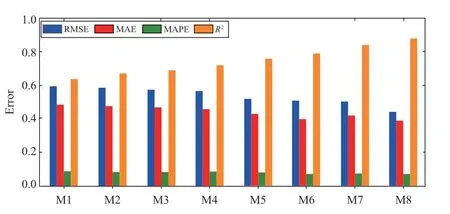
Fig.10 Evaluation metrics for different models (M1: Elman;M2: LSTM; M3: DBN; M4: DBN-Elman; M5: HHT-DBN;M6: HHT-DBN-Elman; M7: IPSO-HHT-DBN; M8: IPSOHHT-DBN-Elman)

4 Conclusion

The WT output is significantly affected by the intermittent and random nature of natural wind and is considered unstable.This hinders the comprehensive development of the wind-power system,seriously affects the stability of the grid system,and is even more unfavorable for the dispatch and control of wind farms.To address the nonlinear and nonstationary nature of wind-speed data,this paper proposed a DBN-Elman combined forecasting model based on IPSO-HHT.

1) To address the problem that the DBN lacks the memory features required for training samples and has a local optimum,a DBN-Elman combined neural network prediction model was proposed.Owing to the strong turbulence and nonlinear characteristics inherent to wind,an improved HHT method was proposed to preprocess the wind speed.

2) Elman was used to optimize the DBN,IPSO algorithm was used to optimize the HHT,and a combined model (IPSO-HHT-DBN-Elman) was established.In the wind-speed prediction test for the wind farm,the prediction accuracy rate was better than that of the other models.

In this study,only the prediction accuracy of the model was considered; the computation time was not.Our future studies will focus on optimizing the structure of the combined model (IPSO-HHT-DBN-Elman) and reducing the computing time.

Appendix A

Table A1 The nomenclatures

Acknowledgements

This study was supported by the Research and Application of Key Technologies in the Design of Large Onshore Smart Wind Power Base (Grant No.XBYZDKJ-2020-05),the Scientific Research Project of the China Electric Power Construction Corporation: Research and Application of Key Technologies in the Design of an Onshore Smart Wind Power Base (Grant No.DJZDXM-2020-52),the Danish Energy Agency (Grant No.64013-0405),the Fundamental Research Funds for the Central Universities (Grant No.B210201018),and the Jiangsu Province Policy Guidance Program (Grant No.BZ2021019).

Declaration of Competing Interest

The authors have no conflicts of interest to declare.