Missing interpolation model for wind power data based on the improved CEEMDAN method and generative adversarial interpolation network

Lingyun Zhao,Zhuoyu Wang,Tingxi Chen,Shuang Lv,Chuan Yuan,Xiaodong Shen,Youbo Liu

1.College of Electrical Engineering,Sichuan University,Chengdu 610065,P.R.China

2.State Grid Sichuan Electric Power Company Chengdu Power Supply Company,610065 P.R.China

3.State Grid Sichuan Electric Power Company,Chengdu 610065,P.R.China

Abstract: Randomness and fluctuations in wind power output may cause changes in important parameters (e.g.,grid frequency and voltage),which in turn affect the stable operation of a power system.However,owing to external factors (such as weather),there are often various anomalies in wind power data,such as missing numerical values and unreasonable data.This significantly affects the accuracy of wind power generation predictions and operational decisions.Therefore,developing and applying reliable wind power interpolation methods is important for promoting the sustainable development of the wind power industry.In this study,the causes of abnormal data in wind power generation were first analyzed from a practical perspective.Second,an improved complete ensemble empirical mode decomposition with adaptive noise(ICEEMDAN) method with a generative adversarial interpolation network (GAIN) network was proposed to preprocess wind power generation and interpolate missing wind power generation sub-components.Finally,a complete wind power generation time series was reconstructed.Compared to traditional methods,the proposed ICEEMDAN-GAIN combination interpolation model has a higher interpolation accuracy and can effectively reduce the error impact caused by wind power generation sequence fluctuations.

Keywords: Wind power data repair; Complete ensemble empirical mode decomposition with adaptive noise (CEEMDAN);Generative adversarial interpolation network (GAIN)

0 Introduction

With the increasing popularity of renewable energy sources,wind power generation has become an important component.However,wind turbines are prone to generating abnormal data during operation,owing to power outages,mechanical failures,and weather-related factors,which have a significant impact on the measurement and prediction of wind power.Therefore,the accurate identification and processing of wind power anomaly data is a pressing issue in the industry.

Currently,interpolation to fill in missing values is considered a common method for handling abnormal data.However,traditional interpolation methods do not adapt well to the characteristics of wind power data,including long time series and unevenly distributed missing values.In addition,these methods cannot guarantee the accuracy and reliability of the interpolation results.Hence,this study aims to explore the causes of abnormal wind power data and propose a new generative adversarial imputation network for repairing abnormal data in wind power generation.

To date,a series of machine learning-based methods have been developed to restore typical time series data(e.g.,wind power).Yang proposed an adaptive neuro-fuzzy inference system (ANFIS) model that used an inference algorithm to interpolate missing and invalid wind data [1].

Huang et al.presented a new data recovery method based on correlation analysis and machine learning to recover the missing wind pressures on the outer walls of high-rise buildings using on-site measurements and structural health monitoring (SHM) [2].Wang proposed a deep neural network (DNN)-based framework for longterm missing wind data recovery and innovatively adopted a frequency spectrum amplitude balancing strategy to enhance the reconstruction of high-frequency components in wind speed signals [3].Additionally,a multivariate time series generative adversarial network (MTS-GAN) was developed by Guo et al.to model the distribution of MTS using multichannel convolution [4].Subsequently,they applied MTSGAN to MTS imputation by formulating a constrained MTS generation task,and the experimental results revealed that MTS-GAN performed well in MTS distribution-modeling experiments [4].

However,these methods tend to be less efficient when utilizing raw data.Traditional neural network interpolation methods can only perform simple replacement or prediction of missing values and cannot learn the distribution and features of the data,thereby leading to potential errors in data reconstruction.Therefore,researchers should focus on developing better structured neural network models for interpolation.

In addition,wind power time series exhibit significant nonlinearity and non-stationarity features,mainly owing to the complex interactions of various factors,such as geographical environment,turbine design,and wind farm operation.Signal decomposition techniques have been widely used to analyze and process power series on wind farms.The multi-step imputation method of “decomposition-imputation of sub-components reconstruction” can effectively improve the final imputation accuracy of the model.

Jin decomposed a monthly MSL time series using the ensemble empirical mode decomposition (EEMD)method.Furthermore,compared to the EEMD method [5],adaptive noise was introduced into the decomposition of CEEMDAN,which improved the accuracy and robustness of the decomposition [5].Ran proposed a hybrid empirical mode decomposition model combining adaptive noise(CEEMDAN) and sample entropy (SE),which achieved excellent results in decomposition tasks [6].

Variational mode decomposition (VMD) is also a common time series decomposition method.Zhao employed the VMD algorithm to decompose and process nonstationary and irregular waves on the east coast of China,followed by time series prediction using a gated recurrent unit deep learning model [7].

Various decomposition methods are widely used in various fields.Nevertheless,traditional decomposition methods such as EEMD and CEEMDAN still suffer from mode mixing,whereas VMD methods require many parameters to be determined during the computation,greatly increasing computational cost of the decomposition task.

In the current study,the CEEMDAN method was improved by introducing an adaptive noise setting that dynamically adjusts the noise level based on the characteristics of the signal.This allows better adaptation to the features of different signals and enhances the effectiveness of signal decomposition.The improved CEEMDAN method was then used to preprocess the wind power time series to improve their non-stationary characteristics.Alternatively a “decomposition-imputation of subcomponents-reconstruction” multi-step imputation method was employed to repair missing data in combination with a generative adversarial network and better results were achieved in wind power missing data repair experiments.

The main contributions of this study are as follows:

1) Considering the non-stationary and fluctuating nature of the wind power time series,an improved ICEEMDAN method was adopted as the preprocessing method for interpolation tasks.

2) In the ICEEMDAN-GAIN interpolation experiment,the ICEEMDAN-GAIN model exhibited a better interpolation performance that other traditional interpolation methods in the same scenario.This contribution offers novel ideas and approaches for advancing research on interpolation methods for missing wind power data that have both theoretical and practical significance.

1 Wind power anomaly data analysis

Various factors may disrupt the normal operation of wind farms,leading to abnormal wind power data [8,9].In the subsequent forecasting process,these abnormal data significantly affect the prediction accuracy of the entire model.Therefore,repairing the original wind power data before forecasting is vital.Figure 1 identifies the three types of data in the original data set of a particular wind farm,normal,missing,and unreasonable.Most the unreasonable data have power values that do not match the actual meteorological conditions,whereas missing data have a power close to zero.

To deal with the actual situation uniformly,the above two types of data (unreasonable data and missing data)are collectively referred to as abnormal data in this study.The following figure shows the approximate proportions of the two types of wind power output data,where the red and green data points represent unreasonable,and missing data,respectively.

To ensure the feasibility and consistency of handling wind power abnormal data,all unreasonable data was processed by being “set to zero,” i.e.,converting unreasonable data to missing data,which were then uniformly imputed via reasonable data imputation method,thus restoring the original wind power data.

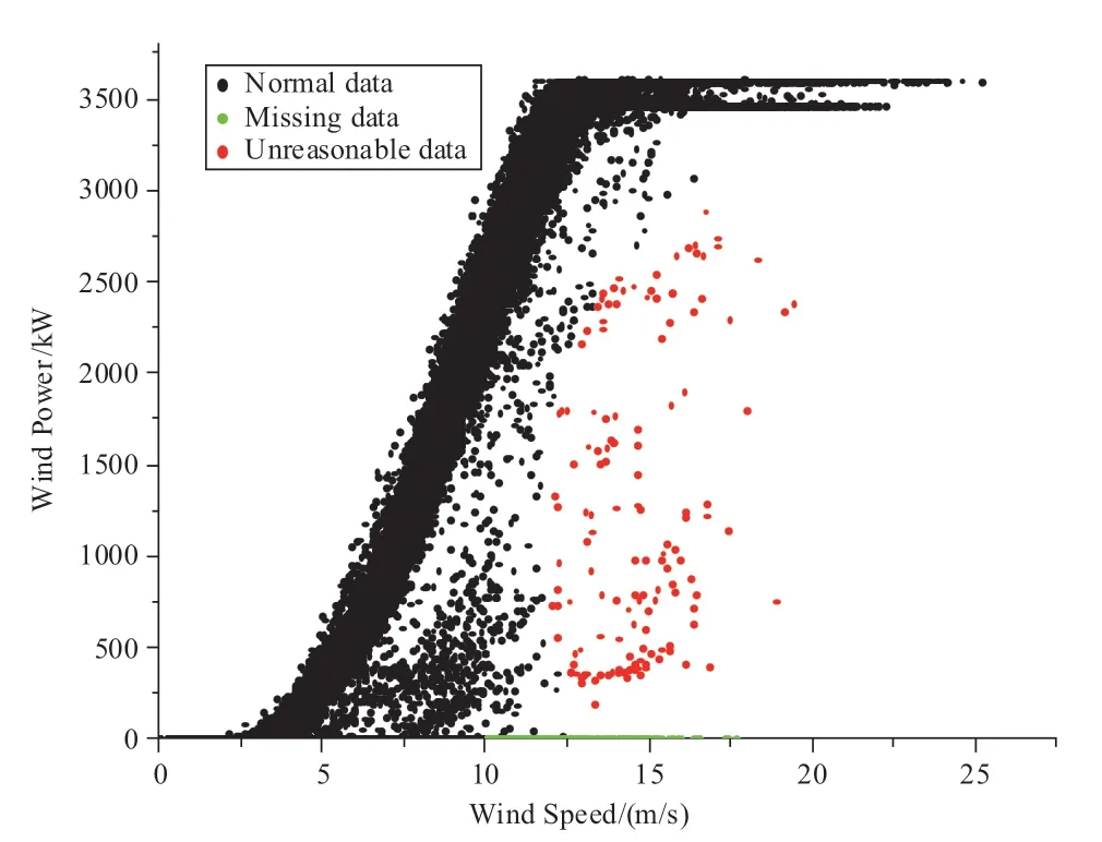
Fig.1 Wind power anomaly data

2 Wind power decomposition preprocessing based on the improved CEEMDAN

2.1 Improved CEEMDAN algorithm

Owing to the uncertainty of meteorological factors such as wind speed and wind direction,wind power time series often exhibit nonlinear and non-stationary characteristics,making their analysis challenging.The CEEMDAN algorithm is a data decomposition algorithm proposed by Torres et al [10,11].The specific decomposition process of the CEEMDAN algorithm is as follows:

1) The CEEMDAN algorithm starts by preprocessing the original signalx(t) by adding Gaussian white noise with zero mean,resulting in a preprocessed sequencexi(t)=x(t) +εδi(t) repeated K times.

In Eq.(1),εis the weighting coefficient of added Gaussian white noise,andδi(t) denotes the Gaussian white noise used for theiexperiment.

2) EMD was performed on the preprocessed sequencexi(t) and the first componentIi1(t) was obtained,and its mean value was taken as the first intrinsic mode function (IMF)componentI1(t) obtained by CEEMDAN decomposition.

In Eq.(2) and Eq.(3),I1(t) is the first IMF component generated by the CEEMDAN decomposition,r1(t)represents thei-th IMF component obtained by the EMD decomposition ofx(t),andr1(t) indicates the residue component obtained after the first decomposition.

3) Gaussian white noise with an average value of zero was added to the residual signal obtained at thejth decomposition stage,and the EMD was continued.

In Eq.(4),Ij(t) represents the j-th IMF component obtained by CEEMDAN decomposition;Ej-1denotes the(j-1)th IMF component obtained by EMD decomposition;εj-1represents the noise coefficient added to the residual component of the (j-1)th stage by CEEMDAN;rj(t) is the residual component of the j-th stage.

4) The above steps were repeated until the number of extreme points in the residual component was decreased to a certain number (usually set to less than or equal to 2)and can no longer be decomposed,then the CEEMDAN decomposition was completed.At this point,the original signal was decomposed into several IMF components and a residual component.

In practice,the CEEMDAN algorithm does not completely solve the problem of mode mixing in its underlying algorithms EMD and EEMD,i.e.,multiple signals of different frequencies are mixed in the same IMF after decomposition.There is still some noise in each component,and pseudo-patterns may exist in each component [12,13].Therefore,based on this,the ICEEMDAN algorithm does not directly use Gaussian noise,but uses the mean of the signal to extract the kthorder mode,minimizing the impact of white noise on mode decomposition.

The decomposition process of the ICEEMDAN algorithm is shown as follows:

1) The first residue signal is calculated using the EMD algorithm:

In Eq.(6),M(·) is defined to represent the local mean of a signal;denotes taking the average.

2) The j-th residual signal and the j-th order modal component can be expressed respectively as:

3) Repeat step 2 until the maximum number of iterations is reached.

2.2 Example of an ICEEMDAN decomposition calculation

EEMD was selected as a comparative algorithm to compare the performance of the improved CEEMDAN method in decomposing the wind power time series.The reconstruction error and modal aliasing phenomena were experimentally compared.In both EEMD and ICEEMDAN,the choice of the number of times and standard deviation of white noise generally requires experience and practice [14-16].In the experiments,the optimal decomposition effect was obtained adding white noise with a standard deviation ranging from 0.01 to 0.5 times that of the original data and a quantity ranging from 150 to 300 instances.

This study used an original wind power data set from a wind farm in Ningxia,China.12 days of data,that is,1152 sampling points,were selected for the decomposition experiment with EEMD and ICEEMDAN with a white noise standard deviation of 0.25 and a total ensemble number of 200 times.

1) EEMD

The default stopping criterion of the EEMD (number of extrema of the residual component less than or equal to one)was applied to decompose the original wind power time series.The results are shown in the following figure,with eight IMF components and one residue component.

According to the EEMD decomposition results,it is clear that the time interval between the peak values of IMF1to r1components gradually increases,indicating that the signal becomes more stable and its complexity gradually decreases as the components are gradually decreased.This phenomenon stems from the observation the high-frequency components and noise are decomposed into the earlier IMF components during the EEMD decomposition process.As the decomposition proceeds,these components are gradually filtered out,leaving the residual component r1 as the more stable signal.

Fig.2 EEMD decomposition results

2) ICEEMDAN

As mentioned previously,unlike the CEEMDAN method,ICEEMDAN addresses the issues of residual noise and spurious modes by utilizing the IMFs obtained from the EMD of Gaussian white noise.This approach not only resolves mode mixing but also significantly reduces the residual the noise within the IMFs.ICEEMDAN demonstrated excellent decomposition and feature extraction capabilities for various scale components contained in wind power time series.

Excessive iterations in ICEEMDAN can result in overdecomposition,leading to the inclusion of more noise and high-frequency IMF components.Therefore,by adjusting the number of iterations through experimental processes,one can effectively select the optimal number of IMF components and avoid over- and under-decomposition.

In the present study,the number of IMFs generated by ICEEMDAN decomposition was adjusted in the range of 3 to 9 to obtain a result set with the smallest modal aliasing and the smallest reconstruction error between each component.After repeated experiments,it was found that by setting the number of IMFs to 5,ICEEMDAN could minimize the reconstruction error and had less significant modal aliasing compared with the EEMD method.The ICEEMDAN decomposition result is demonstrated in Fig.3.

Fig.3 ICEEMDAN decomposition results

The first sequence at the top of each plot represented the original signal.Both decomposition methods generate fewer volatile subsequences; however,the EEMD subsequences have similar trends,whereas the ICEEMDAN sub-sequences have greater differences in trend.The mean absolute error (MAE) was defined,and the equation was

In Eq.(10),Nrepresents the length of the time series,x(t) is the original wind power time series,and,xˆ(t)indicates the reconstructed time series.

Table 1 Reconstruction error

The experimental results reveal that the reconstruction error of the ICEEMDAN algorithm is significantly smaller than that of EEMD,suggesting the effectiveness of the ICEEMDAN algorithm in reducing the impact of spurious white noise and producing superior decomposition results compared to EEMD.ICEEMDAN can further improve the problems existing in EEMD and make the reconstructed signal closer to the true original signal.

For each component sequence,the complexity of the time series can be measured using the permutation entropy[17-19].In this study,embedding dimensionm=3 and time-delayτ=1 were selected,and the permutation entropy of each sub-component in the decomposition results of the EEMD and ICEEMDAN methods were calculated.The permutation entropy was utilized to represent the complexity of the sub-sequences of the two decomposition algorithms.The permutation entropy calculation results for each component are shown in Fig.4.

Fig.4 Permutation entropy of two decomposition arithmetic subsequences

Fig.5 Main structure of GAIN

It can be concluded that the permutation entropy values of each sub-sequence decrease with a decrease in frequency,that is,the non-stationarity of the decomposed sub-sequences gradually decreases and the trend becomes more regular.However,the permutation entropy values of each sub-sequence in the EEMD are close to each other,indicating that some pattern mixing still exists in the subsequences.ICEEMDAN decomposes fewer subsequences and the range of variation in the alignment entropy values is larger.This reveals that there is no evident pattern mixing phenomenon in the sub-sequences.

3 ICEEMDAN-GAIN-based interpolation algorithm for wind power loss

3.1 Generating an adversarial interpolation network

The Generative Adversarial Imputation Network(GAIN),as an improved model based on the GAN,has been extensively applied to missing data interpolation tasks with excellent results [20,21].Unlike other methods,the GAIN does not require complete datasets for model training,but directly uses data with missing values as the model input,and the model output is the imputed complete data.Therefore,the process of GAIN is relatively simple.As a new neural network imputation approach,the GAIN was more suitable than traditional imputation methods for the wind power data in this study.In the GAIN,a binary mask matrixMconsisting of only 0 s and 1 s needs to be established in advance to describe the missing values in the data.The size of the binary mask matrixMis the same as that of the original data setXwithout missing values.An element inMat a position of 0 indicates that the data at the position corresponding toXare missing,and vice versa,with a value of 1.The binary mask matrixMcan be used to label the missing values.By marking the missing positions,these missing values can be handled selectively during data imputation.

The generator usesX,M,and a Gaussian distribution white noise vectorZas the input data.Here,the output of the generatorG(Z) is defined as,that is,the original data are represented asX.The repaired datacan be expressed as follows:

As can be seen from the above equation,the parts of the original data whereXis not missing are retained and the datagenerated by the generator are used to fill in the corresponding missing parts,which are the final repaired data.

GAIN’s overall architecture is shown in the figure above.The generatorGtakes the collected dataX,binary mask matrixM,and Gaussian noise vectorZas input and outputs the dataHere,represents the collected data with missing values.The output data of the generator are expressed as follows:

Compared to the traditional GAN,the guidance mechanism matrix,as the core component of the GAIN structure,was introduced into the GAIN.The purpose of adding the guidance mechanism matrix was to better distinguish the real data from the generated data in the dataset.The bootstrap matrixHis defined as follows:

Eq.(13) illustrates some of the information of the hint matrix containing the mask matrix.The hint matrix is a crucial concept in GAIN.When each element ofM′ is equal to 1,the hint matrixHhas the same information as the mask matrix.However,when all the elements ofM′are zero,the elements ofHare all 0.5.The range of values of the elementshi∈{0,0.5,1} of the hint matrix can be inferred from the above analysis.When the elementhiof the hint matrix was 0,it implied that the input data at the corresponding position of the discriminator is generated data.Whenhiwas equal to 1,the discriminator treated the input data at the corresponding position as real data.When it reached 0.5,no hint information was provided byH,and the discriminator was required to determine the authenticity of the input data independently.

To optimize the GAIN,the generator was first repaired and the discriminator was optimized.The loss function of the discriminator is expressed as

In the above equation,M′ is the predicted value of the mask matrix.

3.2 GAIN Model Interpolation Experiments

In this section,the evaluation metrics of the wind power output test set are compared for different imputation algorithms.The imputation algorithms used include the mean imputation (MEAN),k-nearest neighbor imputation(KNN),missing forest imputation and generative adversarial imputation network imputation (GAIN).

The mean imputation is the most basic imputation method.It uses the average value of all non-missing values of the feature where the missing value is located to replace the missing value.This method is computationally efficient but distorts the empirical distribution of the variables and reduces the variance of the data,making it unsuitable for studying data sets with complex information [22,23].

The KNN imputation algorithm is a widely used data imputation method that identifies neighboring points by calculating distances to judge the similarity between multidimensional data and uses the k most similar values to correct for missing values [24,25].

The missing forest (MF) is a random forest-based imputation method that can handle the missing values of multiple features simultaneously and process non-linear relationships.The missing forest constructs multiple random forests,each of which predicts the missing values based on other features and eventually averages the predictions of the multiple random forests to obtain the final interpolation result.This method has the advantage of handling missing values of multiple features; however,its computational complexity is high and requires a large amount of computational resources.

In practical applications,the value of K in the KNN method should be determined based on factors such as dataset size.In the wind power output dataset used in this study,it was found through comparative experiments in which the optimal data imputation effect could be achieved by setting K to seven.In addition,after multiple comparative experiments,the MF algorithm parameters were set to their values of up to 20 trees and 150 trees per forest.Figure 6 shows the interpolation performance of the four algorithms with missing data rate of 15% and,Table 2 shows the interpolation errors of the four algorithms.

In accordance with the experimental results,it can be found that mean imputation performs well at the data missing rate of 15% as mean imputation simply replaces the missing data point with the average value of the data before and after the missing point in this case.At the same time,the surrounding data is relatively complete and the differences are not significant,so there are relatively small differences between the imputed result and the true value.However,when the missing data rate is high,using average interpolation may lead to larger errors as the interpolation results are affected by larger differences in the surrounding data.Both KNN and MF interpolations are relatively poor and exhibit some errors at the peaks and valleys of the wind power output because KNN needs to select an appropriate number of neighboring points,while MF needs to pre-select features and sample data.In this experiment,the potential of KNN and MF are not realized owing to the small sample size.Compared with the other three imputation methods,the GAIN algorithm exhibits a better performance.This is because it can generate and interpolate data using generators and discriminators in generative adversarial networks.Meanwhile,it can also avoid excessive reliance on the hint matrix for network parameter updates,thereby considering the learning of information for generated data.The imputation experimental errors of the four algorithms with 15% missing data can be noticed in the following table.

As shown Table 2,the highest imputation accuracy was achieved when adopting the GAIN method was adopted.Compared with the MAPE of the mean imputation,KNN,and MF models,the MAPE of GAIN decreased by 24.4%,37.7%,and 31.5%,respectively,and the RMSE decreased by 29.5%,55.9%,and 38.2%,respectively.The GAIN exhibited the highest imputation accuracy.Additionally,it can be seen from the Table 2 that the average interpolation method also has a relatively high interpolation accuracy for the small sample size and a low missing rate was simulated in the above experiments.

The interpolation effect of KNN and MF,as machine learning algorithms,is significantly inferior to that of mean imputation when the missing rate is low.This is because KNN assumes that the similarity between neighbors can be used to fill in missing values; however,in the case of a low missing rate,the correlation between the missing data and neighbors may be weak.This means that when using KNN for imputation,the values of the neighbors contribute less to the imputation of missing data,thereby affecting the imputation effect.On the other hand,MF assumes that the data matrix can be decomposed into two low-rank matrices to reveal the latent distribution characteristics of the data.However,in the case of a low missing rate,the missing pattern of the data matrix may not be evident,implying that the missing data do not have a clear rule or structure for decomposition.This makes it difficult for MF to accurately extract useful information for imputation,thereby affecting the imputation effect.The GAIN method predicts missing values by training a generative model that can comprehensively consider global data for imputation.Even with a low missing rate,the GAIN can improve the imputation effect by following the overall data distribution patterns.Compared with other machine learning methods,GAIN has a clear advantage and outperforms mean imputation in terms of overall performance.

In this series of experiments,the sample size was the same as that used in the previous experiments,with 192 sampling points in 2D.

As shown in Table 3,the RMSE and MAPE of the four data imputation algorithms generally increase as the missing data rate increases.At low missing rates,the accuracies of the mean imputation and GAIN were higher than those of KNN and MF.However,the accuracy of mean imputation was much lower than that of the other three methods at a missing rate of more than 65%,and its performance was not advantageous.From a detailed perspective,at a low missing rate of 20%,GAIN still had the highest accuracy among the four algorithms,which is consistent with the experimental results mentioned earlier,with MAPE being 10.2%,24.8%,and 21.2%,indicating it was less accurate the average interpolation,KNN,and MF,respectively.With a moderate deficiency rate of 55%,GAIN maintained the best interpolation,with 32.1%,29.7% and 18.9% reductions in MAPE compared with the mean interpolation,KNN and MF,respectively.Eventually,for database with high missing rates such as 75%,the data imputation accuracy of the GAN remained high,and the GAN had the best performance among all the algorithms,with a reduction of 45.3%,25.3% and 22.1% in MAPE compared with average interpolation,KNN and MF respectively.The experimental results demonstrate the superiority of the GAIN imputation algorithm proposed in this paper over other traditional imputation algorithms.

The sample sizes of the above experiments were small and the GAIN model may have the following drawbacks in interpolation experiments with small sample sizes:

1) Overfitting: Although the GAIN model reduces overfitting problems using embedded noise,overfitting problems may still exist for small sample sizes.This is because that the model has difficulty in learning complex patterns and relationships in the data,which may lead to inaccurate imputation results.

2) Data distribution: With small sample sizes,data distribution may not be completely or sufficiently representative,leading to biased or inaccurate imputation results from the GAIN model.

In addition,the KNN imputation algorithm is sensitive to overfitting in small sample experiments because it interpolates missing values based on adjacent data points.The MF imputation algorithm uses random forest algorithms for imputation and requires many trees to predict the input data.This can lead to unstable imputation results and decreased accuracy,particularly for small data samples.

Hence,the four algorithms were compared for different sample sizes,with 3,7,20,30,60,and 90 d of wind power data in the comparison experiments.The missing data rate in this series of experiments was maintained at 15%.The experimental results are listed in Table 4.

Table 4 Algorithm interpolation error under different data volumes

As shown in Table 4,the RMSE and MAPE errors of the three data interpolation algorithms,with the exception of the mean interpolation algorithm,generally decreased as the sample size increased.This is because mean algorithm is a simple imputation method that uses only the average value of the variable to fill in the missing values.Additionally,its accuracy was not directly related to the sample size.In cases where training samples are abundant,GAIN demonstrates superiority over mean imputation.Taking the example of 60 d,GAIN reduced the RMSE error by 13.4% compared to mean imputation,and the MAPE error decreased by 45.8%.Similarly,in the case of 90 d,GAIN reduced the RMSE error by 27.4% compared with the mean imputation,and the MAPE error decreased by 51.1%.The lowest MAPE errors of the KNN,MF,and GAIN algorithms were observed for the sample sizes of 60,30,and 90 d,respectively and decreased by 21.62%,26.31%,and 28.69%,respectively,relative to the imputation results of 2 d,respectively.The experimental results verify the improved imputationaccuracy of the KNN,MF,and GAIN algorithms for large sample sizes.

Moreover,regardless of the adequacy of the training samples,the GAIN exhibited a higher interpolation accuracy than the KNN and MF machine learning algorithms,with a more stable performance.Taking a small training sample of 3 d as an example,GAIN reduced the MAPE error by 39.1% compared with KNN and by 30.6% compared with MF.With a large training sample of 90 d,GAIN reduced the MAPE error by 47.7% compared to KNN and by 28.3% compared to MF.In summary,GAIN,as a deep generative model,combines the advantages of generative adversarial networks (GAN) and autoencoders (AE) to generate reasonable interpolation results with enhanced non-linear fitting capabilities.

3.3 ICEEMDAN-GAIN model interpolation process

To address the issue of missing data in wind power time series,this study proposes a missing data imputation scheme based on the ICEEMDAN method and the GAIN network.By default,the GAIN network uses zero values for the initial imputation,however,traditional methods (e.g.,KNN imputation and MF) have different initial imputation conditions.In KNN imputation,the initial imputation value is determined by the observed values of the closest neighbor to the missing value,and the default is to use the mean or weighted mean of the observed values of the nearest neighbor as the initial imputation value.In MF imputation,the initial imputation value for missing values can also include various statistical measures,such as the mean,median,and mode.These statistical measures are usually selected based on factors such as the features and variable types in the dataset,as well as the properties and distribution of the missing values.For data distributions that are not extreme and have no outliers,the unconditional mean is generally used as the initial imputation value in the MF method.

Based on the above rules,a combination imputation model with the initial imputation values is proposed.First,the original missing wind power data were imputed with a mean value to complete the dataset.Subsequently,the data were decomposed into several complete and independent IMF components using the ICEEMDAN method.For each complete and separate IMF component,the two-stage interpolation process of the GAIN network resulted in a final interpolated value with a small error,and the complete wind power time series was subsequently reconstructed.

The basic process of the combination imputation model is as follows:

1) The original wind power signal is obtained.

2) The original wind power signal is imputed with a mean value and decomposed into several IMF components using the ICEEMDAN method.

3) The GAIN model is trained independently and in parallel to perform a second-stage interpolation of the data to obtain the restoration curve corresponding to each IMF component.

4) The imputation output results of all the subcomponents are combined and reconstructed to obtain the final imputation result.

3.4 ICEEMDAN-GAIN model interpolation experiments

In this section,the evaluation metrics of the wind power output test set under the ICEEMDAN-GAIN and EEMD-GAIN algorithms are compared,and the errors of the two algorithms are calculated and compared with the decomposition results from the basic,undecomposed GAIN algorithm.The same two-day data were employed in the experiment as described in the previous section,and the corresponding results of the two algorithms are shown in Fig.8.

Fig.8 Imputation result

The EEMD and ICEEMDAN algorithms decompose raw data into several frequency-stable components,effectively attenuating the volatility and randomness of wind power time series.When the combination interpolation model was used,better fitting results were obtained at the extremal points of the curve.As shown in Fig.8,the ICEEMDANGAIN algorithm can accurately track the fluctuation trend of the wind power output.

Notably,ICEEMDAN-GAIN had the smallest RMSE and MAPE among the three algorithms,with 53.1% and 61.9% decreases in RMSE and MAP respectively compared to GAIN.This is because the multi-step method proposed in this paper first decomposes the signal into multiple subcomponents with different frequency and time-frequency characteristics and these sub-components can be processed separately during the GAIN interpolation process.GAIN can capture the characteristics of each component in the process more accurately,and thus predict the missing data more precisely.The method proposed in this study performed better than traditional single methods in the interpolation of missing data.Second,ICEEMDAN-GAIN decreased the RMSE and MAPE by 50.46% and 61.9%,respectively,compared with EEMD-GAIN.The main reason for this is that CEEMDAN adds noise samples based on EEMD to decrease the noise interference in signal decomposition.This implies that CEEMDAN can better remove the noise component from the signal,during signal decomposition,thereby allowing for more accurate signal components to be obtained.

As shown in Table 6,ICEEMDAN-GAIN and EEMD-GAIN demonstrated a significant improvement in interpolation accuracy compared to GAIN.When the missing rate was low,all the methods exhibited good interpolation performance.However,as the missing rate increased,ICEEMDAN-GAIN exhibited clear advantages.For example,at a 65% missing rate,ICEEMDAN-GAIN reduced the RMSE error by 62.5% compared to the mean imputation,45.4% compared to GAIN,and 25.3% compared to EEMD-GAIN.Similarly,at a missing rate of 75%,ICEEMDAN-GAIN reduced the RMSE error by 49.1% compared with the mean imputation,by 52.4% compared with GAIN,and by 20.2% compared with EEMD-GAIN.Based on the above analysis,ICEEMDAN-GAIN,as a twostage combined interpolation algorithm,effectively captures the temporal characteristics of wind power data and learns the underlying distribution properties of the data,thereby achieving high-quality data interpolation.

In addition,when communication disruptions and sensor failures occur,the wind power data may experience continuous segment loss.Therefore,it is necessary to study the applicability of the ICEEMDAN-GAIN combined method proposed in this paper to continuous data loss throughout the day.In this section,Random selections of 1 d,2 d,3 d,and 4 d were made to simulate continuous data loss,and the corresponding interpolation errors for each time period were calculated.The error results are listed in Table 7.

Under the condition of continuous data loss throughout the day,the mean interpolation and MF methods performed poorly,exhibiting a poor fit to the real data.However,GAIN,as a deep generative model,has the ability to extract hidden temporal information in a sequence,resulting in an overall better interpolation performance than the former methods.Furthermore,ICEEMDAN-GAIN exhibited significant improvements over GAIN and its interpolation performance did not decrease significantly with an increase in the number of missing days.Taking the case of continuous 3-day data loss as an example,ICEEMDANGAIN reduced the MAPE error by 18.3% compared with GAIN.For a continuous 4-day gap,the reduction was 34.3%.This further demonstrates the effectiveness of the proposed algorithm in addressing the issue of missing data on all days.

4 Conclusion

In this study,an interpolation method for missing wind power data based on improved CEEMDAN and GAIN is proposed.Numerical examples prove that the model has smaller result errors and stronger applicability to wind power data sets than traditional methods.

1) In this current study,the causes of abnormal wind power data were first analyzed,the impact of missing wind power data on wind farm operation and power generation prediction was identified and all abnormal data were transformed into the missing data categories through classification and merging.

2) This paper proposes a “decomposition-separate imputation-reconstruction” method for wind power missing data imputation.First,the improved CEEMDAN method was used to decompose wind power into sub-components to decrease its volatility.Subsequently,the GAIN method was used to impute each sub-component separately,and they were reconstructed.The experimental results reveal that the proposed ICEEMDAN-GAIN method has the smallest RMSE and MAPE among the multiple algorithms and a strong imputation ability.

3) The effects of the context similarity loss parameter and hint matrix hint rate parameter on the imputation performance of the GAIN model were investigated.It was proven that,in small sample situations,a larger context similarity loss weight and an appropriate hint rate can achieve better results in the imputation experiment.

However,there are some limitations to the ICEEMDAN-GAIN method.For example,for extreme missing situations,such as a highly uneven distribution of missing data,the effectiveness of the proposed model may not reach an ideal level.This can be addressed by further improving the model structure or by conducting additional data preprocessing.This should be considered account in the future studies.

Acknowledgements

We gratefully acknowledge the support of National Natural Science Foundation of China (NSFC) (Grant No.51977133 & Grant No.U2066209).

Declaration of Competing Interest

The authors have no conflicts of interest to declare.