Multi-Objective Optimization for an Industrial Grinding and Classification Process Based on PBM and RSM
2023-10-21XiaoliWangLumingLiuLianDuanandQianLiao
Xiaoli Wang, Luming Liu, Lian Duan, and Qian Liao
Abstract—The grinding and classification process is one of the key sub-processes in mineral processing, which influences the final process indexes significantly and determines energy and ball consumption of the whole plant.Therefore, optimal control of the process has been very important in practice.In order to stabilize the grinding index and improve grinding capacity in the process,a process model based on population balance model (PBM) is calibrated in this study.The correlation between the mill power and the operating variables in the grinding process is modelled by using the response surface method (RSM), which solves the problem where the traditional power modeling method relies on some unobservable mechanism-related parameters.On this basis, a multi-objective optimization model is established to maximize the useful power of the grinding circuit to improve the throughput of the grinding operation and improve the fraction of –0.074 mm particles in the hydrocyclone overflow to smooth the subsequent flotation operation.The elite non-dominated sorting genetic algorithm-II (NSGA-II) is then employed to solve the multi-objective optimization problem.Finally, subjective and objective weighting methods and integrated multi-attribute decision-making methods are used to select the optimal solution on the Pareto optimal solution set.The results demonstrate that the throughput of the mill and the fraction of –0.074 mm particles in the overflow of the cyclone are increased by 3.83 t/h and 2.53%, respectively.
I.INTRODUCTION
THE grinding-classification process is an important link in mineral processing, and its performance plays a decisive role in the economic and technical indexes of the whole plant[1].Modeling and optimization of industrial grinding-classification processes has always been a focus of researchers and engineers [2].
Process indexes in the grinding-classification circuit often refers to the throughput and particle size in the overflow of the classification operation, etc.[3], [4].Momayaet al.[5] successfully applied a model predictive control (MPC) method to an industrial lead-zinc grinding operation, which solved the explicit optimization problem of maximizing throughput and kept the passing percentage of midsize fraction within user specified bounds.Chenet al.[6] proposed a supervisory expert control strategy to stabilize the particle size of the product and improve the throughput in ball milling circuits.The characteristic of this method is that the proportion of the desired size fraction is stable as throughput increases.Brookset al.[7] combined two typical MPC structures of ball milling and flotation.In this model, the milling MPC reduced throughput to ensure finer grinding and made the response of the ball milling controller react smoothly and in a coordinated fashion.Ziolkowskiet al.[8] simulated a semi-autogenous grinding mill with extreme seeking control (ESC) to maximize the fraction of the specified size of the mill using grinding curves [9], but this method could not control the throughput.The above studies show that particle size and throughput are often in contradictory in actual production.Therefore, in order to simultaneously optimize these two indexes, multiobjective optimization (MOO) becomes a key technique in the modeling and optimization of the grinding process.
Traditional MOO methods often transform the MOO problem into a single objective problem by establishing an evaluation function [10], [11].However, these methods are difficult to apply in the optimization of grinding processes.In recent years, the intelligent optimization algorithm has become a hot research topic in the field of grinding [12].Mitra and Gopinath [13] adopted the NSGA-II [14] to optimize the grinding operation of an industrial lead-zinc concentrator to improve the yield and the pass rate of the most important particle size.Mitra and Majumder [15] used NSGA-II to solve a multi-objective optimization task (simultaneous maximization of throughput and tumble index) of an industrial iron ore induration process too.Farzanegan and Vahidipour [16] combined the genetic algorithm (GA) with a grinding circuit simulator (BMCS) to optimize the predefined process objective(e.g., specific d80 circuit output).Dinget al.[17] proposed a hybrid differential evolution algorithm based on orthogonal design and an archiving mechanism and applied it to the optimization of a mineral processing process.Yuet al.[18] proposed a new multi-objective nonlinear programming model for the optimization of production planning and decomposition (P & D) to improve concentration output, grade and concentration ratio, and to reduce metal recovery and production cost.In order to improve the quality of the solutions and the speed of searching, a hybrid evolutionary algorithm is proposed based on an interactive partition (IP) and multi-objective gradient (MO-G).A steady-state multiple reactors gradient optimization strategy, unsteady-state operational pattern adjustment strategy, and a process evaluation strategy based on oxidation-reduction potential are proposed [19].A multiobjective optimization approach based on the state transition algorithm [20] and constrained nondominated sorting algorithm is proposed to find optimal solutions.
Although the conflict between overflow fineness and mill capacity in the grinding classification process has been discussed in the existing literatures, most of the researches just focused on the improvement and application of multi-objective optimization methods.And when dealing with the above two performance indexes, it is always achieved by maximizing the grinding feed and product quality objectives.However,the relationship between mill capacity, mill load and power is rarely considered.Some studies suggest that within a certain range, the active power of the mill increases with the increase of load, and then decreases with the increase of load after reaching a certain boundary which can be regarded as the optimal point of the mill load [21], [22].Therefore, to some extent, the peak area of mill power means that the state of mill load reaches an optimal value, which corresponds to the optimal processing capacity, and has the best working efficiency.When the mill is at its best working efficiency, the utilization rate of energy is the highest.Therefore, in this study, an industrial grinding-classification process is optimized by using the MOO method to improve the mill load and the particle size index, and save energy.Here, the particle size index means the mass fraction of particles smaller than 0.074 mm (denoted as –0.074 mm) in the overflow of the classificaton operation.
The rest of this paper is arranged as follows.The industrial grinding-classification process is described in Section II and a process model is established in Section III.In Section IV, a method which is different from analysis of mill structural parameters or internal state of the ball mill (as example in[23]) is used to establish an energy model, and a data-based mill power model is established, which reflects the relationship between adjustable input variables and mill power, and solves the problem where the traditional power modeling method relies on some unobservable mechanism parameters.The multi-objective optimization model, the analysis of the Pareto optimization frontier and the optimal setting values selection method through multi-objective decision-making methods are described in Section V.The conclusions are discussed in Section VI.
II.PROCESS DESCRIPTION
The industrial grinding process studied in this paper is shown in Fig.1, which consists of an overflow-type ball mill and a set of cyclones.In the process, the crushed raw ore and water are fed into the ball mill at a certain ratio.Water is also added to the ball mill discharge to maintain the required concentration of the slurry.The discharge slurry flows into a sump called the primary sump and then is pumped to the bank of primary cyclone.Underflow of the primary cyclone is recycled and overflow is sent to the secondary grinding process.The particle size distribution obtained by the grinding circuit is significant to the performance of the subsequent flotation process, which makes the operation of the grinding circuit essential for the entire processing operation.Meanwhile, the plant hopes to maximize throughput and minimize energy and steel consumption to improve economic efficiency.Due to the complex process behavior and strong coupling variables, the grinding circuit is difficult to maintain under optimal operating conditions.The interrelation of production objectives makes the trade-off between grinding quality and throughput necessary.Therefore, modelling, optimization and control of the grinding circuit performance are significant.
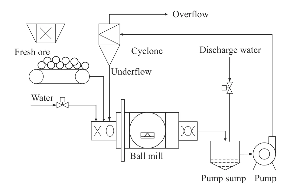
Fig.1.A single-stage closed-circuit grinding classification circuit.
III.OVERFLOW PARTICLE SIZE MODEL BASED ON PBM
In this section, a hybrid ball mill model and a cyclone model are calibrated.The model parameters are associated with key operating parameters including a ball filling ratio (br, %),flowrate of fresh ore fed to the mill (Fo, t/h), flowrate of water fed to the mill (Fw, m3/h) (called feed water), inlet pressure of cyclone (Ph, Mpa) and the flowrate of water fed to the discharge (Fd, m3/h) (called discharge water) to implement the prediction of product quality in the first-stage grinding classification process under a normal working state.
A. Ball Mill Model
The ball mill model is established based on the population balance framework [24], where the product size distribution is calculated as
whereiandjare the size-interval indexes running up ton;i=1represents the coarsest particles andi=nrepresents the finest particles.piis the mass fraction (%) of the particle size intervaliin the mill product,dijis a transformation matrix describing the breakage of the feed into the discharge product,andfiis the mass fraction of sizejin the feed.The expression ofdijis shown in (2)-(4),
wherebijis the fraction of sizejmaterial which appears in sizeion primary breakage,Siis the specific rate of breakage of a material with sizei.Φ(τ) is the residence time distribution(RTD) function.RTD describes the transportation of materials through the mill.It can be approximately simplified as one large/two small fully mixed reactor-series model.Then, (4)becomes (5),
whereτ1= 0.25τis the mean residence time of the large reactor, andτ2= 0.25τis the mean residence time of the two small reactors [24].Mean residence time τ is determined by the fresh ore feed flowrate and the concentration inside the ball millCm.Cmis related to the operating variables of the mill,includingFo,Fw, andFd, as defined in the first paragraph of Section Ⅲ.The empirical functions are shown in (6) and (7),
wherecis the circulating load.
The breakage distribution functionBijis the cumulative form ofbij, which is as follows:
whereB11= 1.Bijis only related to the properties of the ore,and basically irrelevant to the grinding conditions.The four parametersb1,b2,b3andb4are regarded as constants.The specific rate of breakageSiruns in the following form [25]:
wherexirepresents theith particle size, and in general,x0= 1.In the above formula,μis a parameter proportional to the mill diameter and the maximum ball diameter.It is treated as a constant in this work.ais related to the ball filling ratio (br).αand Λ are parameters related to material properties and operating parameters.The material property parametersAandBare regarded as constants, and the operating parameters are the feed flowrate of fresh ore and flowrate of feed water, respectively.The correlations betweenα, Λ and working condition variables and feed distribution was established as in (11)-(13)by using regression [26]
B. Cyclone Model
The operating effect of the cyclone is mainly evaluated by classification efficiency, that is, the ratio of the amount of each particle size interval entering the underflow to the amount of the corresponding particle size interval in the feed[27].The formula is shown in (14),
whereEiis the classification efficiency (%) of theith size interval;diis the particle size (mm) of theith interval;d50cis the corrected cut size (mm) which is the size of the material with equal probability to enter the underflow and the overflow only due to the classification effect;mserves as a direct measure of the sharpness of classification;Rwis the water ratio (%) which represents the amount of water in the feed pulp entering the underflow.The above three parameters are related to the mass concentration (%) of the cyclone feedCw,the volume concentration (%) of the cyclone feed slurryCvand the volume flow (m3/h) of the cyclone feedQ[28], the parameters in the equations were identified using 22 groups of data collected from the industrial process and the relationships are
Cw,CvandQare related to the flowrates of fresh ore (Fo),feed water (Fw) and discharge water (Fd).The first-stage cyclone model is shown in (18),
whereaciandpiare the mass percentage of theith size interval in the overflow and in the mill discharge, respectively.
C. Validation of the Models
50 groups of samples, including the ball mill discharge and the overflow of the cyclone, were collected at a different time from the industrial process and sieved by using a standard Taylor screen.The actual content of the –200 mesh (0.074 mm) in the mill discharge and the corresponding calculated values by the model are shown in Fig.2(a).The bar chart in Fig.2(b) shows that the maximum relative error is 8.60%.
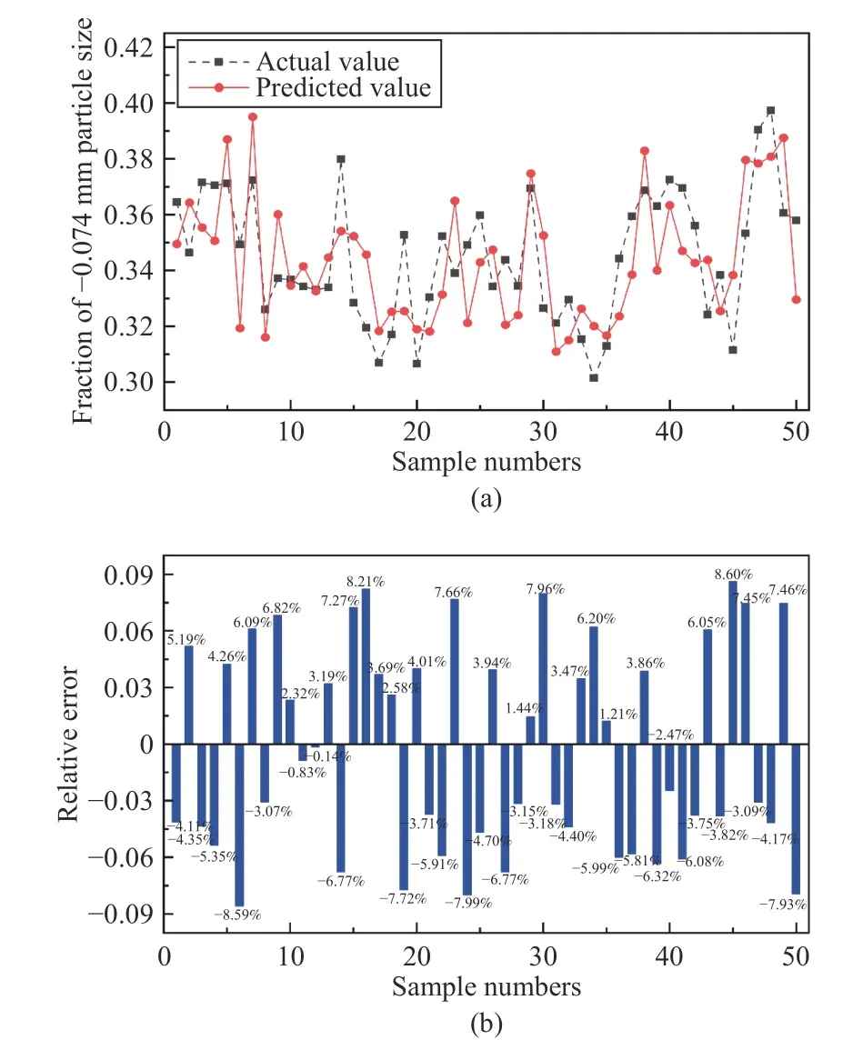
Fig.2.Primary ball mill (fraction of -0.074 mm particle size): (a) Comparison between actual value and predicted value; (b) Relative error.
The validation of the fraction of -0.074 mm in the overflow is shown in Fig.3, where the maximum relative error is 8.88%.
IV.MILL POWER MODEL BASED ON RSM
In this section, RSM is used to establish the relationship between mill power (Pmill) and three operating variables including ball filling ratio (br, %), fresh ore feed (Fo, t/h) and feed water (Fw, m3/h).
A. Central Composition Design
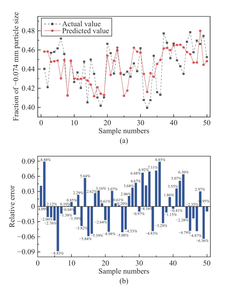
Fig.3.Primary cyclone (fraction of -0.074 mm particle size): (a) Comparison between actual value and predicted value; (b) Relative error.

TABLE I INDEPENDENT VARIABLE VALUES AND THEIR CORRESPONDING LEVELS
Central composition design (CCD) has been extensively used for a multivariate nonlinear regression model to explore the interaction of several parameters affecting the process[29].All variables are coded into five levels (-α, -1, 0, +1,α),as shown in Table I.The actual levels of the three variables for CCD are shown in Table I.The upper level of the ball filling ratio is the maximum filling ratio when two bags of steel balls are added for many consecutive days, and the lower level is the filling ratio when one bag of steel balls is added for many consecutive days and then after one day of wear.The fresh feed is set to 150 t/h.Considering of the fluctuation within a large range of production, the upper limit of feed is 167 t/h, and the lower limit of feed is 133 t/h, +17 from a central point.The upper and lower limits of water fed to the mill are 67 m3/h and 33 m3/h, respectively.That is, under the premise of considering most production conditions, the range of milling concentration is 66.5%~83.5%.
The total number of CCD schemes consists of 2kfactorial points, 2kstar points andnccentral points, wherekis the number of variables.Considering that there are three variables, the number of central points isnc= 8, and 22 groups of data with factorsbr,Fo, andFw, under appropriate combination are obtained, which can cover different levels of the three factors.Meanwhile, the corresponding response valuePmillis obtained from the distributed control system (DCS) with a varying range from 1226 to 1410 kW.
B. Results of RSM With CCD
The 22 groups of process data were fitted to a full quadratic second order model equation by applying multiple regression analysis forPmill.The model is shown in (19).
To confirm the reliability of the quadratic model and to identify the significance of the influence of each variable on the response, the model was analyzed by analysis of the variance (ANOVA) (5% significant level).The P-value and Fvalue evaluated the significance of the correlation between the variables and the response, as shown in Table II.

TABLE II RESULTS OF ANOVA
It can be seen from Table II that F-test value isF= 146.42,P< 0.0001 < 0.01, indicating that the model is extremely significant.The misfit term of this modelP= 0.1055 > 0.05,indicating that the loss of fit term in this model is not significant.The results show that the prediction model of mill power can better reflect the relationship between the three selected variables and the output response.The goodness of fit of the model can be verified by the determination coefficientR2and the modified determination coefficientRadj2.The closer theR2is to 1, the better the fitting degree of the model is.For the power modelR2= 0.991, which shows that there is a strong correlation between the predicted values and the actual values.Radj2= 0.9242, indicating that the model can explain 92.42%of the variability.The above data analysis shows that the power model established by the CCD method is effective.
The model adequacy verification test diagram is shown in Fig.4.The true power value measured by experiment is basically consistent with the power value predicted by the RSM model as shown in Fig.4(a).In Fig.4(b), all the power test values obtained in this test follow a normal distribution without deviation variance.Figs.4(c) and 4(d) show that the externally studentized residual range of all test points and Cook’s distance in the model are all within the range of +3.95 and 0.91, respectively.The results show that there is no abnormal value of power obtained under the test condition.In conclusion, it is further verified that the RSM model is reliable in predicting power value.
Next, combined with the actual production situation, the influence of the three variables and their interaction terms on the mill power response is discussed from the perspective of the model.The influence degree of the variables on the response value can be determined by the value ofF.In Table II,F(br) = 712.93,F(Fo) = 299.24,F(Fw) = 6.06, which shows that the significance of the input factors isFo>br>Fw.According to Table II, the primary termsbrandFoof the regression equation have an extremely significant impact on the mill power (P< 0.001 < 0.01), andFwhas a significant impact on the mill power (P= 0.0299 < 0.05).The secondary termbr2,Fo2andFw2are extremely significant to the mill power (P< 0.001 < 0.01); the interaction termsbrFohave an extremely significant impact on the mill power (P< 0.007 <0.01), andFoFw,brFwhave no significant influence on mill power.
The influence of single variable on mill power is discussed in Fig.5.Fig.5(a) is a perturbation diagram showing the influence of each variable on power when other factors remain at their respective midpoint level.It can be visually seen that compared to the other two variables, the ball filling ratio has the most significant influence on the power response.Figs.5(b)–5(d) show the influence trend of each single variable on mill power when other variables are at the central level.As shown in Fig.5(b), when the steel ball filling ratio is at a low level, i.e., 25%–34%, the mill power increases with the increase of ball filling ratio, and the curve steepness of power gradually flattens and tends to decrease with the increase of ball filling ratio.As shown in Fig.5(c), when the feed is lower than 160 t/h, increasing of the fresh feed is equivalent to increasing of the mill load.When the feed reaches about 160 t/h, the mill load is the highest, and the power will decrease with the increase of fresh feed.Fig.5(d)shows that when the water fed to the mill changes, the change range of the power value is very small.The power increases first and then decreases with an increase of feed water.The above single variable impact analysis is consistent with the results in [30].
In order to establish the general relationship between each factor and the response, based on (19), the model results are drawn as a 3D response surface map and contour map (the projection of response surface on two-dimensional plane), as shown in Fig.6.

Fig.4.Performance visualization of the Mill power model: (a) Comparison between the real and the predicted value; (b) Normal probability; (c) Comparison of residual and operation; (d) Cook’s distance (colors are arranged by run).

Fig.5.Analysis of single factor: (a) Perturbation diagram; (b) Variation of mill power with br; (c) Variation of mill power with Fo; (d) Variation of mill power with Fw.

Fig.6.Response surface and contour map: (a) and (b) The influence of fresh ore feed and ball filling ratio on mill power; (c) and (d) The influence of ball filling ratio and feed water on mill power; (e) and (f) The influence of fresh feed and feed water on mill power.
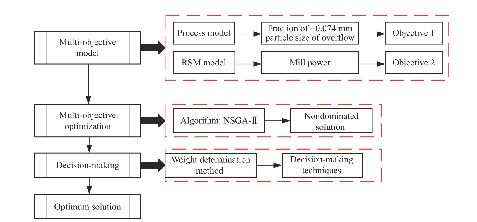
Fig.8.Flowchart of the multi-objective model and decision-making method.
Fig.6 shows the results when one variable is fixed at the central level, and the other two variables interact.Figs.6(a) and 6(b) show that when the ball filling ratio is low (25%-28%),the power increases with the increase of fresh feed.When the ball filling ratio is high (30%-32%), the power increases first and then decreases with the increase of fresh feed, so that the fresh feed with the best power is about 158 t/h.Figs.6(c) and 6(d) show that when the ball filling ratio is at a low or high level, the increase of feed water has little impact on the change of power.On the contrary, when the water fed to the mill is at a low (about 35 m3/h) or high (about 60 m3/h) value,the ball filling ratio is about 30%, and the mill power reaches the best value.As can be seen from Figs.6(e) and 6(f), the contour shape of the two factors tends to be circular, indicating that the interaction is not significant.When the water fed to the mill and fresh ore feed are around the central horizontal position, that is, when the water fed to the mill is about 50 m3/h and the fresh feed is 150–155 t/h, the power reaches the best value.
C. Power Model Verification
In order to verify the effectiveness of the power model under actual continuous production, 8 days of production data are collected from the DCS system with a total of 10 978 groups of data.The raw actual power values and the predicted values are shown in Fig.7(a).The filtered actual power values and the predicted values are shown in the Fig.7(b).The average relative error is 0.39%.Fig.7(c) is an enlarged view of a section with 200 data points, which has the average relative error of 0.57% and the maximum relative error of 0.73%,as shown in Fig.7(d).
Therefore, the power model based on RSM method can well reflect the actual process production.
V.SYNCHRONOUS OPTIMIZATION OF GRINDING PROCESS QUALITY AND CAPACITY BASED ON NSGA-II
A. Multi-Objective Optimization Model
In order to optimize product quality and process capacity in the process of grinding and classification, a multi-objective model was established.Then NSGA-II which is a widely used method to solve MOO problem is applied to find a group of non-inferior solutions.Finally, a group of optimal operation values are obtained from the non-inferior solutions using decision-making methods.The structure of the model and optimization is shown in Fig.8.
The fraction of the -0.074 mm particle size in the overflow is taken asf1to reflect grinding quality, and the mill power is taken asf2to reflect the corresponding mill capacity.According to the prediction models in Sections Ⅱ and Ⅲ, the input variables of the multi-objective optimization model are the ball filling ratio (br), flowrate of fresh feed (Fo), flowrate of feed water (Fw), spiral flow inlet pressure (Ph) and discharge water supplement (Fd).Production practice shows that the grinding concentration (Cm) has a significant impact on product quality, that is, the lower or higher theCmis, the worse the productivity and product quality are.Therefore,Cmshould be controlled within a certain range,f2should be stable above the minimum value andf1should not be smaller than an expected value.The multi-objective optimization problem of grindingclassification process is then described as follows:
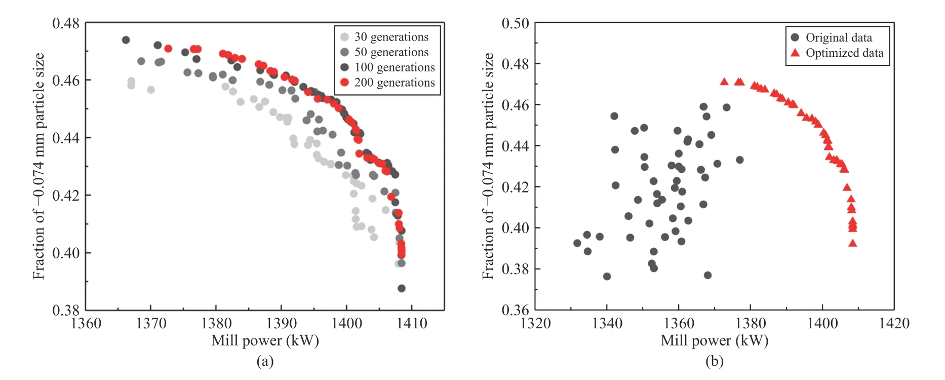
Fig.9.Optimization results: (a) Pareto front under different iterations; (b) Comparison between the optimized data and the original data.
where superscriptLandUdenote the lower and the upper bounds of the above variables.
B. Optimization Model Solving Results and Discussions
We conducted simulation experiments on 50 groups of real production data to verify the effectiveness of the optimized setting values obtained in this paper.Fig.9(a) shows the twodimensional projection diagrams Pareto solution sets for the NSGA-II algorithm at 30, 50, 100 and 200 iterations.It shows that with the number of iterations increases, the distribution of the Pareto front gradually moves to a better position and becomes denser, which means that the NSGA-II can effectively find the better solution sets.The distribution ranges of the Pareto solution set corresponding to 100 and 200 iterations are basically consistent.Thus, the Pareto set converges when the generations are 100.
The on-site data and the Pareto fronts found at the generation number 200, for normalized objective functions, are given in Fig.9(b).The parameter setting used to run NSGA-II is as follows: crossover rate is 0.1, mutation rate is 0.2, simulated binary crossover parameter is 2 and polynomial mutation parameter is 5.As shown in Fig.9(b), “●” denotes the original data collected from the process without optimization, and“▲” denotes the optimization results in this paper.According to the goal of maximization, the closer a solution is to the right or upper area, the better it is.In production, the performance of the process depends heavily on the experience of operators in feeding of balls, ores and water, which makes it difficult to maximize the overflow fineness and mill capacity at the same time.Fig.9(b) shows that the original setting value is located on the left and below the optimization results,which means that the optimized setting value is better than the original empirical setting value.
Fig.10 shows the comparison of fineness, power and feed values of the 50 samples before and after optimization.Table III shows the numerical comparative analysis.It shows that the overflow fineness is increased by 2.53% on average and by 6.04% on relative average.The optimized fraction of the-0.074 mm size reaches 80.00%.The mill power is increased by 40.46 kW on average and by 0.98% on relative average.The set value of mill capacity is increased by 3.83 t/h and 2.55% on average and relative average, respectively, and the maximum optimization improvement is 11.71 t/h.
According to the relationship between the power and the load of the mill, the mill power increases with the increase of the mill load.When it reaches the optimal area of the mill load, the mill power reaches its maximum value.As the load continues to increase, the power of the mill shows a downward trend, that is, the maximum of the useful power reflects the optimal value of the mill load.Fig.11 is the power level diagram corresponding to the mill load before and after optimization.These experimental results show that the mill power increases with an increase of the load within a certain range.By comparing the load increment and power increment of the mill, it is found that when the load increment is relatively large, the corresponding useful power increment is also relatively large, and the overall fineness of -0.074 mm in overflow shows an optimal trend.Therefore, on the premise of ensuring the stability of overflow fineness, increasing mill power can increase the capacity of the mill to a certain extent.
C. Decision Making on the Optimization Solutions and Discussion

Fig.10.Performance visualization: (a) Comparison of overflow fineness measured and optimized values; (b) Comparison of mill power measured and optimized values; (c) Comparison of mill fresh feed measured and optimized values.

TABLE III COMPARISON BETWEEN ORIGINAL DATA AND DETERMINED OPTIMIZATION DATA

Fig.11.The mill power and the flowrate of fresh ore before and after optimization.
A set of Pareto solutions is obtained by solving the multiobjective optimization problem with the results in Section V.It is necessary to make a decision on this set of solutions in order to obtain an optimal solution suitable for the problem.The multi-objective optimization problem is composed of two attributes: mill power (MP) and product quality of the primary overflow (POF), which is used to evaluate and rank the points in the Pareto front.Considering that there are only two evaluation attributes in this paper, the multi-attribute border approximation area comparison (MABAC), the technique for order preference by similarity to ideal solution (TOPSIS) and the compromise ranking method (VIKOR), which are usually used as multi-criteria decision-making (MCDM) techniques,are investigated in this study.The main differences between these methods are the sorting scheme, the decision mechanism, and the aggregation function.Among them, the methods to determine weight are the subjective weight method and objective weight method.Fig.12 illustrates the weight vector as stacked bars obtained by AHP (integrated analytic hierarchy process), EW (entropy weight) and GRA (grey relational analysis) methods [31].
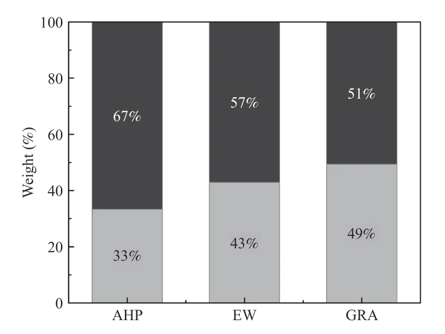
Fig.12.Weight vectors obtained by different methods (the dark color represents the weight of attribute POF and light color represents the weight of attribute MP).
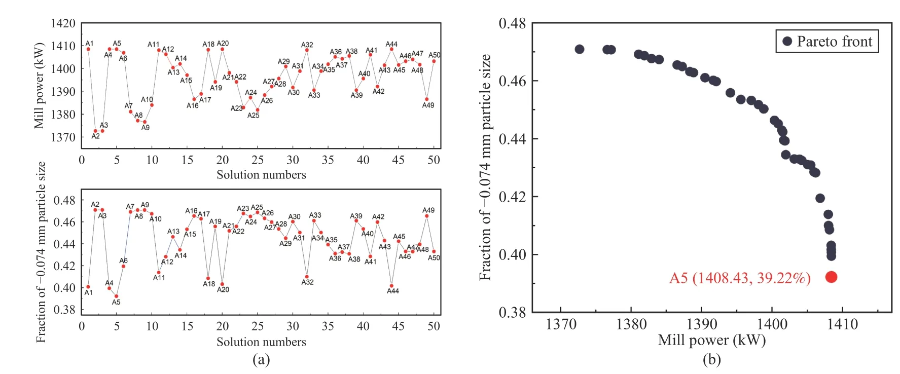
Fig.13.NSGA-II algorithm optimization results: (a) Information of the Pareto front solutions; (b) The Pareto front and the optimal solution.
Based on the optimization results obtained by the NSGA-II algorithm, the optimized values of the two criteria can be determined, as shown in Figs.13(a) and 13(b), and the Pareto front is composed of 50 candidate solutions.
Table IV shows the optimum solutions selected from the best Pareto front by using the three decision-making techniques and the three weight-determination methods, respectively.

TABLE IV DECISION RESULTS
TOPSIS method chooses solutionA10(1383.99, 46.73%)under the three weighting methods.MABAC chooses solutionA5(1408.43, 39.22%) under the subjective weighting method AHP, because this method depends on the distance from each weighting scheme to the approximate area.The POF attribute described in the pairwise comparison matrix obtained by the AHP weighting method is more important than the MP attribute, so the optimal decision tends to find the optimal value of overflow fineness.And MABAC chooses solutionA3(1372.69, 47.09%) under the other two objective weighting methods.The VIKOR method obtains compromise solution through mutual concession to maximize group effect and minimize individual loss.This method analyzes the information of the solution under the objective weighting method and selects solutionA13(1400.35, 44.63%), while under the subjective weighting method, it selects solutionA5(1408.43,39.22%).
Considering different decision-making techniques, the optimal decision-making solution can be selected fromA10andA5.The decision variables of solutionA10are as follows: the fresh feed is 151.10 t/h, the water fed to the mill is 41.06 m3/h,the spiral flow inlet pressure is 0.06 Mpa, and the discharge water supply is 99.69 m3/h.The decision variables of solutionA5are as follows: the fresh feed is 158.17 t/h, the feed water is 52.60 m3/h, the spiral flow inlet pressure is 0.05 Mpa, and the discharge water supplement is 73.21 m3/h.In addition to these differences,A10andA5presented the same ball filling ratio of 0.3.
If the fraction of -0.074 mm particle size in overflow can meet the expected product quality, we can consider reducing the requirements for the fineness content in overflow to improve the ore feeding capacity of the mill, so as to improve the grinding efficiency.Therefore, solutionA5can be selected as the optimal set points of the ball filling ratio, fresh feed,water fed to the mill, spiral flow inlet pressure and discharge water supply.
VI.CONCLUSIONS
In order to stabilize the grinding index and increase mill capacity in the process of grinding classification, a hybrid model for particle size prediction is calibrated and a RSM model for mill power is proposed.On this basis, a multiobjective optimization problem is constructed to precisely find the optimal operating setting values of grinding-classification.Then NSGA-II is applied to get the solution set.Finally, the best operating setting values were found through a multiple decision-making method, which effectively utilizes production experience and expert knowledge.Our study can be concluded as follows:
1) Considering of the influence of grinding conditions on the useful power of the mill, a mill power response surface model of fresh mill feed, water fed to the mill and discharge water flowrate is established based on process data, which solves the problem where the traditional power model relies on some unobservable mechanism-related parameters.This model can precisely reflect the relationship between adjustable variables and power, and therefore reflects the load state of the mill.
2) A MOO problem is constructed to search for optimal values of operating variables for an industrial polymetallic grinding operation.The objective function is used to simultaneously maximize the mass fraction of -0.074 mm particle size in the primary overflow and the ball mill power.NSGA-II algorithm is applied to solve the multi-objective optimization problem.The optimization results demonstrate that the throughput of the mill and the fraction of -0.074 mm in the overflow of the cyclone are increased by 3.83 t/h and 2.53%,respectively.
3) By combining the subjective and objective weighting method and three other decision-making methods, the most suitable operation set-points for the grinding-classification process are found: ball filling ratio is 0.3, flowrate of the fresh mill feed is 158.17 t/h, flowrate of feed water is 52.60 m3/h,inlet pressure of the hydro-cyclone is 0.05 Mpa and flowrate of discharge water is 73.21 m3/h.These experimental results provide a meaningful set point for the grinding circuit control.
The actual environment of the grinding-classification process is complex and changeable, and the modeling and optimization process is easily affected by uncertain factors.Therefore, in our future work, we will consider the uncertain optimization of the grinding-classification process to improve the robustness of the set point of the grinding-classification process.
杂志排行
IEEE/CAA Journal of Automatica Sinica的其它文章
- Containment-Based Multiple PCC Voltage Regulation Strategy for Communication Link and Sensor Faults
- GraphCA: Learning From Graph Counterfactual Augmentation for Knowledge Tracing
- Adaptive Graph Embedding With Consistency and Specificity for Domain Adaptation
- The ChatGPT After: Building Knowledge Factories for Knowledge Workers with Knowledge Automation
- An Optimal Control-Based Distributed Reinforcement Learning Framework for A Class of Non-Convex Objective Functionals of the Multi-Agent Network
- Can Digital Intelligence and Cyber-Physical-Social Systems Achieve Global Food Security and Sustainability?
