Iterative Regularization Method for the Cauchy Problem of Time-Fractional Diffusion Equation

LV Yong(吕拥),ZHANG Hongwu(张宏武)

(School of Mathematics and Information Science, North Minzu University,Yinchuan 750021, China)

Abstract: We consider a Cauchy problem of the time-fractional diffusion equation,which is seriously ill-posed.This paper constructs an iterative regularization method based on Fourier truncation to overcome the ill-posedness of considered problem.And then,under the a-prior and a-posterior selection rules of regularization parameter,the convergence estimates of the proposed method are derived.Finally,we verify the effectiveness of our method by doing some numerical experiments.The corresponding numerical results show that the proposed method is stable and feasible in solving the Cauchy problem of time-fractional diffusion equation.

Key words: Cauchy problem;Time-fractional diffusion equation;Iteration regularization method;Convergence estimate;Numerical simulation

1.Introduction

The time-fractional diffusion equation is deduced by replacing the first-order time derivative with the derivative of fractional order,and which has the important applications in describing the various anomalous diffusion phenomena.In the past few decades,the forward problems for time-fractional diffusion equation have been studied extensively.[1-3]In recent years,driven by practical applications,the inverse problems of this equation have attracted wide attention.The research contents mainly include the parameter identification problem,inverse initial value problem (final value problem or backward problem in time),Cauchy problem,sideways problem (inverse heat conduction problem),inverse source problem,inverse boundary condition problem,and so on.

This paper considers the Cauchy problem of time-fractional diffusion equation

andΓ(·) is the Gamma function.

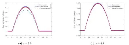
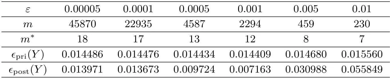
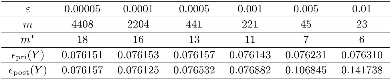
The physical background and motivation for the problem(1.1)can be described as below.In practical scientific research,the solute concentration of the pollution in soil at internal point and one endxLare not available to be measured since the internal point is inaccessible or the end ofxLis far away,but the solute concentration and diffusion flux can be measured at another endx0.Our task is to determine the unknown solute concentrationY(x,t)(0

There are two main difficulties in solving the above problems.(i)Problem(1.1)is ill-posed in the sense that the solution does not depend continuously on the noisy datumωδ(t),µδ(t),so some regularized methods are required to overcome its ill-posedness and recover the stability of the solution.(ii) The Caputo derivative in time-fractional diffusion equation possesses the properties of weak singularity and non-locality,this can lead to some difficulties in the aspect of numerical computation,then in order to solve problem (1.1),one needs to design a stable discretization scheme to complete the numerical computation and simulation.In order to recover the stability of the solution and obtain the stable numerical solution for Cauchy problem of time-fractional diffusion equation,recently some works have been published,in which some meaningful regularized methods and numerical algorithms have been proposed.For example,spectral regularization and finite difference method[5],convolution type regularization and finite difference method[6],modified Tikhonov regularization and finite difference method[7],Tikhonov regularization and boundary element method[8],modified Tikhonov regularization and conjugate gradient algorithm[9],kernel-based approximation method[10],truncation-type regularization[11],etc.

In the present paper,we propose an iterative regularization method based on Fourier truncation to recover the stability of solution for the problem(1.1).And then,the a-prior and a-posterior convergence results for this method are given and proven.Finally,in consideration of the properties of weak singularity and non-locality of Caputo derivative,we solve a direct problem to construct the exact datum by adopting an unconditionally stable finite difference scheme proposed in [2],and use the fast discrete Fourier transform and inverse transform to compute the regularized solution.Meanwhile,we verify the calculation effect of our method by doing some numerical experiments.Numerical results show that this method works well in doing with the problem (1.1).On other references for the similar iteration methods,we can see [12-16],etc.

The rest of this article is arranged as below.Section 2 gives a mathematical description for the considered problem.Section 3 describes the ill-posedness of Cauchy problem and the construction procedure of iterative(or regularized)method.Section 4 derives the a-prior and a-posterior convergence results of regularization method.Section 5 verifies the calculation effect of our method by doing some numerical experiments.Some conclusions and further discussion are shown in Section 6.

2.Mathematical Formulation of the Cauchy Problem

Let2(R),Fourier transform and inverse Fourier transform are defined as

Since we shall work with Fourier transform with respect to the variablet,we extend the domain of appearing functions with respect totby defining them to be zero for(−∞,0).

According to the principle of linear superposition,as in [7],problem (1.1) can be split into the following two Cauchy problems:

ForR,by using Fourier transform with regard tot,the solutions of (2.3),(2.4) in the frequency domain can be expressed as

Using the inverse Fourier transform,the exact solutions of (2.3) and (2.4) respectively can be expressed as

From (2.5) and (2.6),the solution of (1.1) in the frequency domain is as below

the exact solutionY(x,t)u(x,t)+v(x,t).

Further,we assume that there exists a constantE>0 such that the solutions of (2.3)and (2.4) satisfy the a-priori bound

where,∥u(L,·)∥p,∥v(L,·)∥pare both Sobolev spaceHp-norm defined by

3.The Iteration Regularization Method

Ⅰ The iteration regularization method for Problem (2.3)

Take the initial guess as zero,if utilizing the original Landweber iteration method[17],we know that the iteration solution(regularization solution)of(2.3)in the frequency domain can be written as

Ⅱ The iteration regularization method for Problem (2.4)

Adopting the same procedure,for the problem (2.4),we also can construct the original Landweber iteration solution as

4.Convergence Estimates for a-priori and a-posteriori Rules

In this section,we choose the iteration numbermby the a-priori and a-posteriori rules and derive the convergence estimates for our method.We give two inequalities which can be proven by the knowledge in real analysis.We shall use them to prove the convergence of iteration method.

Lemma 4.1[12]Let 0≤s ≤1,m ≥1,then the following results hold

Ⅰ The a-priori convergence estimate

Theorem 4.1(The a-priori convergence estimate for solving Problem (2.3)) Letugiven by (2.8) be the exact solution of the problem (2.3) with the exact dataω,andbe the iteration solution defined by(3.3)with the measured datawδwhich satisfy(1.4).Suppose that the a-priori condition(2.11)is satisfied.If choosing the iteration step numberm[E/δ],then for fixed 0

ProofFrom Parseval equality and the trigonal inequality,we have

Similar with the procedure of [7],it can be easily proven that the following inequalities hold

Firstly,we use the a-priori condition (2.11) and the inequalities (4.2),(4.5) and (4.6),and it can be obtained that

Combining the above two estimates onJ1,J2and (4.4),it can be derived that

Next,we use the similar method to derive the a-priori convergence estimate for the method in the problem (2.4).

Theorem 4.2(The a-priori convergence estimate for solving Problem(2.4)) Letvgiven by(2.9)be the exact solution of problem(2.4)with the exact dataµ,andbe the iteration solution defined by (3.6) with the measured dataµδwhich satisfy (1.4).Suppose that the a-priori condition (2.11) is satisfied.If we choose the iteration step numberm[E/δ],then for fixed 0

ProofSimilar proof process to(4.5)and(4.6),we can prove that the following inequalities hold

Meanwhile,note that

Using the a-priori condition (2.11) and the inequalities (4.2),(4.8) and (4.9),it can be obtained that

According to the above two estimates onJ3,J4,we can derived that

Based on the conclusions in two theorems above,we can give the a-prior convergence result of our method when it is used to solve the problem (1.1).

Corollary 4.1 LetY(x,t) be the exact solution of problem (1.1) with the exact dataω(t) andµ(t),is the iteration solution with the noisy dataωδ,µδwhich satisfy (1.4),and assume that the a-priori condition (2.11) is satisfied.If we choose the iteration step numberm[E/δ],then for fixed 0

whereC3C1+C2.

Ⅱ The a-posteriori convergence esimate

We know that the a-priori stopping rule for iteration number (regularization parameter)needs the a-priori boundEof exact solution.However,a-priori bound generally can not be known,this often brings a lot of inconvenience to the actual calculation.Below,we select the iteration number by the a-posteriori stopping rule,here it does not depend on the a-priori boundEof exact solution,and depends on the noisy levelδand measured datumωδorµδ.For the general theory on the a-posteriori selection of regularization parameter,we can see the Morozov discrepancy principle[18].

For the iterative scheme in (3.2),we control the iterative step numberby

whereτ>1 is a constant,denotes the first iterative step which satisfies the inequality of(4.12).

ProofFirstly,J1andJ2are similar to (4.4),from the proof process of Theorem 4.1,we know that

Meanwhile,from the iteration scheme (3.2) and the a-posteriori stopping rule (4.12),it can be obtained that

According to the above two estimates onJ1,J2,we can derived that

Below,we give the a-posteriori convergence estimate for solving Problem (2.4).For the iterative scheme (3.6),we control the iterative step numberby

whereτ>1 is a constant,denotes the first iterative step which satisfies the inequality of(4.16).

Meanwhile,from the iteration scheme (3.5) and the a-posteriori stopping rule (4.16),it can be obtained that

Finally,based on the results in two Theorems above,we give the a-posteriori convergence estimate of our method when it is used to solving the problem (1.1).

Remark 4.1Note that,based on the ill-posedness analysis and iteration method in this paper,the following iterative scheme for solving problem (2.3) can also be constructed

Similarly,the iterative scheme for solving the problem (2.4) can be designed as

5.Numerical Implementations

In this section,the feasibility and effectiveness of the proposed method are verified by several numerical examples.LetL,T>0,in order to do numerical experiments,we restrict the problem in a bounded domainG(0,L)×(0,T).Since explicit exact solution is difficult to be constructed,we consider the direct problem

and the boundary condition

The Neumann data for Cauchy problem (1.1) can be constructed by

The measured data is generated by the random perturbation from

whereε1denotes the noisy level ofω,ε2denotes the noisy level ofµ,the corresponding measured error bound is calculated byδε1∥ω∥+ε2∥µ∥.

For the fixedx,we calculate the relative error between the exact and iteration solutions by

Example 5.1In the direct problem(5.1),we takew(t)1−e-2tandg(t)2 sin(8πt).It is clear thatg(t) is a smooth function,and it belongs toHp(R)⊂L2(R).To verify the effect ofpon the error results,atx1,ε0.001,α0.01,the relative errors and iterative step numbers for variouspare presented in Tab.1.Next we will selectp2 to do the numerical experiment.Since∥Y(L,·)∥H2∥g(t)∥H2894.0026<895,we takeE895.Forε0.001,p2,α0.1,the exact and iteration solutions atx1.0,0.3 are shown in Fig.1.Forε0.001,p2,α0.01,the exact and iteration solutions atx1.0,0.3 are shown in Fig.2.Atx1,p2,α0.01,the relative errors and iterative step numbers for various noisy levelεare presented in Tab.2.

Fig.1 At x=1.0,0.3, p=2, E=895, α=0.1,the exact and iterative solutions for ε=0.001

Tab.2 At x=1, p=2, E=895, α=0.01,the relative errors and iterative step numbers for various ε

Example 5.2In the forward problem (5.1),we takeω(t)0,and

We know thatg(t) is a continuous function,but it only belongs toH1(R)⊂L2(R).Note that,∥Y(L,·)∥H1∥g(t)∥H1<1,so we choose the a-priori bondE1.Forε0.001,p1,α0.1,the exact and iteration solutions atx1.0,0.3 are shown in Fig.3.Forε0.001,p1,α0.01,the exact and iteration solutions atx1.0,0.3 are shown in Fig.4.Atx1,p1,α0.01,the relative errors and iterative step numbers for various noisy levelεare presented in Tab.3.

Fig.3 At x=1.0,0.3, p=1, E=1, α=0.1,the exact and iterative solutions for ε=0.001

Fig.4 At x=1.0,0.3, p=1, E=1, α=0.01,the exact and iterative solutions for ε=0.001

Tab.3 At x=1, p=1, E=1, α=0.01,the relative errors and iterative step numbers for various ε

Example 5.3In the forward problem (5.1),letω(t)1−e-t2,and

We know thatg(t) is a discontinuous function,it does not belong toHp(R),but it belongs toL2(R).Note that,∥Y(L,·)∥L2∥g(t)∥L2<2,we choose the a-priori bondE2.Meanwhile,in order to verify the simulation e ect of iterative method,we still takep2 to calculateξ1.Forε0.001,p2,α0.1,the exact and iteration solutions atx1.0,0.3 are shown in Fig.5.Forε0.001,p2,α0.01,the exact and iteration solutions atx1.0,0.3 are shown in Fig.6.Atx1,p2,α0.01,the relative errors and iterative step numbers for various noisy levelεare presented in Tab.4.

Fig.5 At x=1.0,0.3, p=2, E=2, α=0.1,the exact and iterative solutions for ε=0.001

Fig.6 At x=1.0,0.3, p=2, E=2, α=0.01,the exact and iterative solutions for ε=0.001

Tab.4 At x=1, p=2, E=2, α=0.01,the relative errors and iterative step numbers for various ε

Tab.1 shows that,phas no significant effect on the numerical results.From Figs.1-6 and Tabs.2-4,we can see that our iteration method is stable and feasible in doing with the smooth and non-smooth cases.Figs.1-6 show that numerical results become worse asxapproaches to 1,this is mainly because the given data point (x0) is far away from the inversion point (x1),it is a common phenomenon in solving inverse problems of partial dierential equation.Meanwhile,it can be concluded that as the orderαdecreases,the calculation effect becomes well.Tabs.2-4 indicate that,as the iteration step numbermincreases,the calculation error of each example is gradually stable.

6.Conclusions and Further Discussions

This article studies a Cauchy problem of the time-fractional diffusion equation.This problem is ill-posed in the sense that its solution is instable.We constructed an iterative regularization method to overcome its ill-posedness and derived the prior and posterior convergence results,respectively.Meanwhile,by making some numerical experiments we also verify the effectiveness of our method in doing with the smooth and non-smooth cases.Numerical results show that the proposed method is stable and feasible in solving the considered problem.

We point out that this paper mainly investigates the regularization theory and algorithm for problem(1.1),but not considers the conditional stability.In 2011,[19]used the Carleman estimate to establish a stability result for a special time-fractional diffusion equation(the orderα1/2) in bounded domain.In 2014,[7] derived a stability estimate of Hölder type,but this result is invalid for the endxL.Therefore,it is quite necessary to establish an optimal stability result that can be valid for all 0

AcknowledgmentsThe authors would like to thank the reviewers for their constructive comments and valuable suggestions that improve the quality of our paper.The work was supported by the NSF of Ningxia (2022AAC03234),the NSF of China (11761004),the Construction Project of First-Class Disciplines in Ningxia Higher Education(NXYLXK2017B09)and the Postgraduate Innovation Project of North Minzu University (YCX22094).