Deep learning for estimation of Kirkpatrick-Baez mirror alignment errors

Jia-Nan Xie · Hui Jiang · Ai-Guo Li,3,4 · Na-Xi Tian · Shuai Yan · Dong-Xu Liang · Jun Hu

Abstract A deep learning-based automated Kirkpatrick-Baez mirror alignment method is proposed for synchrotron radiation.We trained a convolutional neural network (CNN) on simulated and experimental imaging data of a focusing system.Instead of learning directly from bypass images, we use a scatterer for X-ray modulation and speckle generation for image feature enhancement.The smallest normalized root-mean-square error on the validation set was 4%.Compared with conventional alignment methods based on motor scanning and analyzer setups, the present method simplified the optical layout and estimated alignment errors using a single-exposure experiment.Single-shot misalignment error estimation only took 0.13 s,significantly outperforming conventional methods.We also demonstrated the effects of the beam quality and pretraining using experimental data.The proposed method exhibited strong robustness, can handle high-precision focusing systems with complex or dynamic wavefront errors, and provides an important basis for intelligent control of future synchrotron radiation beamlines.

Keywords Deep learning · Synchrotron radiation · Optics alignment

1 Introduction

Synchrotron micro- or nano-focused X-rays have been widely used to explore the microstructures of materials in the fields of energy [1] and material and life sciences [2].For a coherent source, smaller focusing spots yield higher coherent fluxes, improving the resolution of the reconstructed images.To meet the high demand for X-ray focusing systems, aberration-free focusing systems are desired for perfect wavefronts.The Kirkpatrick-Baez (KB) mirror pair is a typical X-ray focusing system [3, 4] consisting of two perpendicular mirrors with elliptical or parabolic shapes.To achieve an ideal focusing spot, in addition to the highprecision surface figure, KB mirrors must be placed accurately along the optical axis.Conventionally, a KB mirror is aligned by trial and error.A knife-edge scan [5] is the simplest method for measuring the focusing spot size; however,it can only provide one-dimensional (1D) intensity profile information in one scan.The Hartmann wavefront sensor[6] can provide two-dimensional (2D) wavefront information directly in one shot; however, the device is expensive and has a relatively low spatial resolution.Grating-based shearing interferometry [7, 8] is another approach to obtaining 2D wavefront information; however, these measurements require accurate alignment of interferometers and nearly perfect fabrication of gratings.Recently, a near-field speckle-tracking method [9] based on digital image correlation (DIC) was developed for extracting wavefront information, and relevant characteristics of this method, such as the effect of the diffuser grain size [10] and correlation subset size [11], were carefully explored.A speckle-based scanning method was also proposed to directly provide information on the pitch angle error [12]; however, the scanning process is time-consuming, and the acquired alignment information is limited to the pitch angle and wavefront curvature.Another speckle analysis method [13] based on coherent X-ray beams was developed for obtaining alignment error-related information in one shot based on the inverse relationship between the speckle and focusing spot sizes.A few more shots were required to attenuate the noise in this method.

In recent years, the rapid development of deep learning has extended to the field of optical systems.A convolutional neural network (CNN) was trained for estimating the Zernike coefficients of wavefront aberration using a pre-conditioner to increase the number of informative pixels in the detected image [14].A deep residual wavefront learning method was also proposed to extend the usable range of Lyot-based loworder wavefront sensors [15].Instead of using images as the network input, Tchebichef moments were introduced to extract the features of point-spread functions (PSFs)and passed to a multiple neural network (MNN) [16].In the telescope field, a CNN was used for determining the initial estimates of the Zernike coefficients from the PSF images [17] for further iterative refinement.In microscopic systems, deep learning has been used for autofocusing[18, 19] and denoising [20].In the field of X-rays, neural networks have been used for screening macromolecular X-ray crystallographic diffraction images [21], classification of crystal structures [22], tomographic denoising [23], and Bragg peak analysis [24].Machine learning-based methods have also been applied to the diagnosis and tuning of accelerators [25, 26].However, relevant applications of deep learning in X-ray optics alignment and metrology remain lacking.

In this study, we propose a single-exposure deep learningbased KB mirror alignment error estimation method.We use the detected images to train a CNN for estimating alignment errors.To improve the performance of the deep learning methods, we place a thin scatterer in the focal plane to modulate the direct beam and generate speckles in the detector plane, because these speckles can carry the wavefront error-related information of the focal plane.We first train the CNN using simulated data and then use experimental data to fine-tune the network.The influence of the beam quality and pre-training with simulated data on the misalignment error estimation is also discussed.

2 Method

As shown in Fig.1, a thin scatterer was placed in the focal plane to generate speckles in the direct beam images on the detector as a modulation (pre-conditioner) for training the CNN.Unlike other image-based machine learning methods,we used both direct beam and speckle-modulated images for training the network to extract the features of the detected images and compared the performance of the network on them.

For a narrowband incident light wave,u(P,t), the mutual intensity can be defined asJi(P1,P2) =u(P1,t)u*(P2,t).After passing through a thin scatterer with a complex transmittance functiont(P), the exit mutual intensity becomesJt(P1,P2) =t(P1)t*(P2)Ji(P1,P2).The propagation of the mutual intensity from the scatterer surface S1to the detector surface S2can be written as [27]

Fig.1 (Color online) Schematic of the experimental optical path using with the proposed method

whereλrepresents the center wavelength of the narrowband beam,riis the distance betweenPiandQi, andχ(θi) is the obliquity factor at positionPi.

Because only the intensity information can be detected, we considerI(Q) =J(Q,Q) in the detector plane.Let (x,y) denote positionQin the detector plane, and let (α,β) denote positionPin the scatterer plane.By assuming a Schell model fieldJi(α1,β1,α2,β2) =A(α1,β1)A(α2,β2)μ(α1-α2,β1-β2) and using the Fresnel approximation, we obtain the following simplified expression:

wherezindicates the output of a given layer,wandbrepresent the weight and bias parameters of individual neurons of this layer, respectively,xis the input to this layer (also the output from the previous layer),Lis the loss function reflecting the optimization objective, and constructs such as

As indicated by the above equation, the scatterer perturbs the detected intensity.Using deep learning methods, we can extract the speckle difference owing to the scatterer by learning together the detected images with and without scattering.Deep learning methods use backpropagation and gradient descent for optimizing the parameters of artificial neural networks.A typical artificial neural network contains many layers of neurons.Each layer receives the output of the previous layer as input and feeds processed input to the next layer; the last layer outputs the model predictions.The gradient of the loss function capturing the difference between the model predictions and ground truth is propagated backward through the network starting from the output layer, according to the backpropagation algorithm.Specifically, for a layer of neurons,the forward and backward propagation rules are as follows:∂L/∂xare backpropagation gradients formulated as Jacobian matrices.

For image processing, CNNs have become much more popular than vanilla multilayer neural networks, according to some recent advances in deep learning.Compared with conventional multilayer neural networks, CNNs leverage the ideas of local connectivity, parameter sharing, and pooling of hidden units.Thus, they are more computationally efficient, exploit the 2D topology of image pixels, and account for translation invariance.The backbone CNN in the present study was ResNet50 [28] (schematically shown in Fig.2), which demonstrated good performance on various vision tasks and has been a popular backbone network for many types of vision-related tasks.We added a dropout layer with a drop ratio of 0.2 to mitigate the overfittingproblem; in addition, we added a fully connected layer for regression.

Fig.2 (Color online) Schematic of the misalignment error estimation process.Dropout: dropout layer.FC: fully connected layer.Conv: convolution layer

3 Simulation results

Considering the sensitivity of the different alignment errors associated with KB mirrors, we focused on six main degrees of freedom: (1, 2) vertical and horizontal pitch angles, (3, 4)vertical and horizontal curvatures, (5) astigmatism, and (6)defocus.Single-micron focusing was pursued based on the experimental environment.

First, a simulation was performed to verify the feasibility of the proposed method.The optical layout and photon energy of 10 keV were the same as in the experiment in beamline BL15U (more detailed information is provided in Sect.4), as shown in Fig.1.The simulation was conducted in 1D for horizontal and vertical focusing first, then combined to form a 2D focus by shearing and matrix multiplication,and finally was propagated to the detector plane to reduce the computational complexity.The source was simulated using an array of point sources with a random phase sampled from a uniform distribution within a preset range.Based on the diffraction fringes generated by the source and the relationship between the contrast of the fringes and coherence length of the Gauss-Schell model, the transverse coherence length values at the source position were measured as less than 3 μm horizontally and 42 μm vertically in simulations(averages over one thousand replicates).A thin scatterer was simulated using five layers of randomly distributed 500-nmsize Cu particles, as shown in Fig.3a.The particle sizes were drawn from a Gaussian distribution (mean, 500 nm;standard deviation, 0.25 of the mean).The tangential figure of the KB mirrors was simulated using an elliptical curve with randomly added high- and low-frequency errors.Highfrequency figure errors were drawn from a Gaussian distribution (root-mean-square (RMS), 0.2 nm; peak and valley(PV), 1 nm), while low-frequency figure errors were drawn using a sin function of a complete cycle with a 30-nm PV and a random initial phase.Medium- or low-frequency figure errors yielded coherent stripes in far-field images, different from lower-frequency alignment errors.To overcome a possible alignment error-related estimation bias introduced by figure errors, the mirror figure was not fixed in the simulations; for each generated figure, the simulation was repeated 10 times, and a new figure was generated and used.An example error curve is shown in Fig.3b.The lengths of the horizontal focusing mirror (HFM) and vertical focusing mirror (VFM) were both 200 mm to simulate the KB mirrors used in experiments.The ideal focus size without alignment errors was approximately 1 μm in both directions.

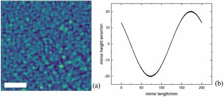
Fig.3 (Color online) Example simulated optical elements.a Simulated scatterer composed of Cu particles and b simulated figure error of the KB mirror.Scale bar: 20 μm

The tolerances for the six main misalignment parameters were estimated using the Strehl ratio based on the Marechal criterion, using the simulation results.The Strehl ratio averaged over 100 simulations with a random source field sampled from a uniform distribution, and the corresponding results are listed in Table 1.

For better reliability and robustness, we also added deviations of other degrees of freedom to the simulations as experimental noise to avoid overfitting to an ideal environment; these errors included the error of the detector position,roll angle error, and beam in-/out-axis error (the distance that the mirror moved from the optical axis in the tangential plane).We did not include the roll angle error in the estimation because the simulation program was unable to simulate comprehensive 2D interaction of the beam and mirrors,which led to the focus insensitivity to the roll error, and the proposed experimental platform was unable to adjust the roll angle between mirrors.This perpendicularity error can be easily included in the estimation by adding a dimension to the output of the last FC layer, if required.The simulation was implemented according to the optical layout shown in Fig.1, and 8000 samples were generated using the simulation program for machine learning, one of which is shown in Fig.4.Owing to the 1D simulation of the KB focusing process, the vertical and horizontal beam propagations were decoupled, and there was an obvious correlation between the detected images for different directional points, owing to the matrix multiplication of the focus field.The alignment parameters and error ranges are listed in Table 2, where the errors were randomly drawn from a uniform distribution.The range of the estimated errors was chosen to enlarge thefocal spot to approximately 10 μm; the range of the errors acting as noise was chosen to not visibly affect the size of the focal spots.

Table 1 Estimated tolerances for six main alignment parameters

Fig.4 (Color online) Example simulated speckle (a) and direct beam (b) detector images.Scale bar: 1 mm

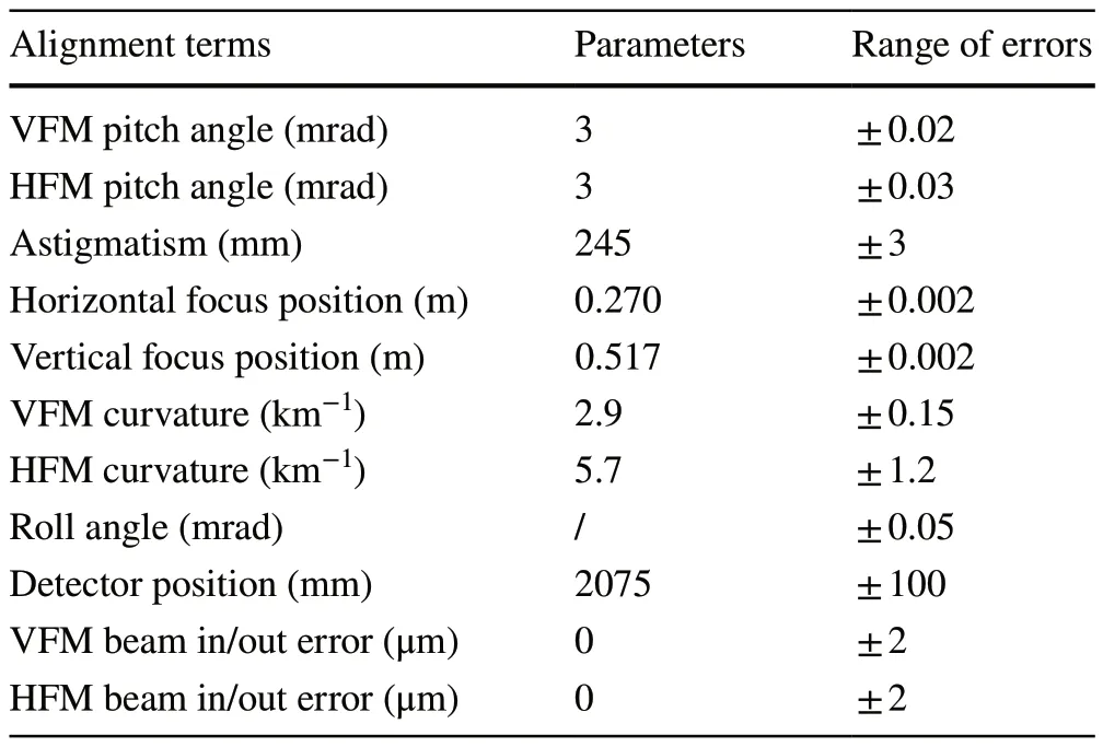
Table 2 Alignment parameters and ranges of misalignment errors in the simulations

We used the Adam optimizer [29] for training our CNN,because it generally converges faster than the stochastic gradient descent (SGD) method.The learning rate was 10-4, with a rate of decrease at 0.978 per epoch.The batch size was 10, and the training was performed for 80 epochs.Gaussian noise with a signal-to-noise ratio (SNR) of 50 dB was added to the images to simulate a practical noise environment for further robustness.The misalignment errors were normalized to the [- 1, 1] range as the target value to avoid gradient explosion or imbalanced weights among the estimated errors.The loss function was the mean square error (MSE), commonly used in regression tasks.The method was implemented in PyTorch and executed on an NVDIA A100 GPU with 40 GB of VRAM.

The training was performed using three different datasets: speckles, direct beams, and both.We combined the speckle and direct beam images in different channels for training.The results are listed in Table 3, and the training results for the speckle dataset are shown in Fig.5.The RMSEs between the ground truth and estimated alignment errors for the test datasets were 0.271 ± 0.126 for the combined dataset of speckle and direct beam images,0.265 ± 0.122 for the dataset of speckle images, and 0.273 ± 0.126 for the dataset of direct beam images, while the corresponding RMSEs for the training datasets were 0.05, 0.045, and 0.047, respectively.Overfitting occurred early during training, and the RMSE of the test dataset decreased slowly approximately from epoch 10, as shown in Fig.5c.While the RMSE of the training error continued to decrease to 0.045 over the entire training process, the RMSE of the validation error stopped at approximately 0.3 and started to oscillate around it with a small amplitude.This happened because the randomness of the incident beam status and mirror figure strongly affected the features of the detected images; for one set of misalignment error parameters, the detected images generated in the simulations varied strongly in the case of different statuses of the incident beam and mirror figures.Increasing the amount of data or using a constant phase for the incident beams and mirror figures may relieve this problem.The best performance was obtained for the speckle dataset.Combining the images from the speckle and direct beam datasets did not utilize the advantages of both datasets, and the resultant performance was similar to that obtained usingonly the dataset with direct beam images.Among the six parameters, astigmatism and defocus were the main contributors to the RMSE of the alignment error.Because these two parameters spanned small ranges compared with the large depth of focus, the detected images had low sensitivity to changes.

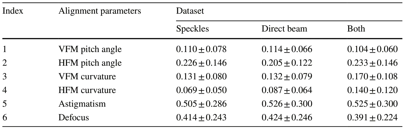
Table 3 Summary of validation accuracies (RMSEs) of normalized misalignment error estimation models trained on the simulated data

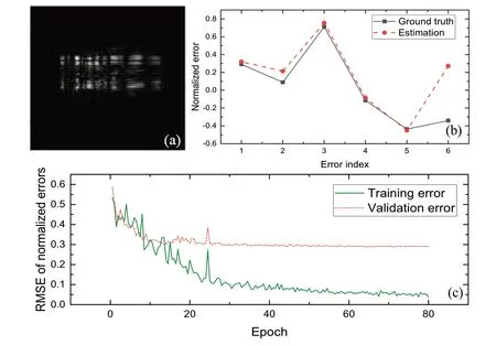
Fig.5 (Color online) Results of training the network on the speckle data.a A detected image generated by the simulation.b The corresponding estimation.c The RMSE drop during the training process.Error indices: (1) VFM pitch,(2) HFM pitch, (3) VFM curvature, (4) HFM curvature, (5)astigmatism, and (6) defocus

Compared with the estimation of the Zernike wavefront coefficient, the proposed method directly obtains information about the misalignment of KB mirrors rather than inferring the misalignment from the wavefront phase information provided by the Zernike coefficients and wavefront amplitude information calculated from the intensity information of the detected images.By using an end-to-end misalignment estimation model, this method introduces fewer calculation errors.

4 Experimental results and discussion

The experiment was conducted at the beamline BL15U of the Shanghai Synchrotron Radiation Facility (SSRF), using photons with the energy of 10 keV.The secondary source aperture was 200 μm × 30 μm for improving the beam coherence, and the coherence lengths at aperture were 4.25 μm in the horizontal direction and 66.55 μm in the vertical direction [30].Bendable KB mirrors (active length, 200 mm)were pre-aligned with a silicon substrate at the beamline.The slope error along the optical axis of the KB mirrors was less than 0.5 μrad, and the roughness of the surfaces coated with Pt and Rh layers was at least 0.3 nm RMS.The ends of the mirrors were equipped with two bending rods above and below the surfaces, for applying the bending force, and two fixed rods were used to support and stabilize the mirrors.The curvatures of the KB mirrors were adjusted using actuators attached to the benders.A thin sandpaper scatterer was placed at the focus.A microscope objective lens system (Optique Peter) coupled to a complementary metaloxide semiconductor (CMOS) camera (Hamamatsu) was placed 2075-mm downstream from the focus.The detector pixel size was 1.625 μm, and there were 2048 × 2048 pixels.To pass their values to our CNN, we cut the image from the beam center to reduce the space occupied by the background and downsampled it to 500 × 500 pixels, considering the computational ability of the network.The position of the minimal spot size based on the knife-edge scan results was considered the zero-error position for the alignment.Although the theoretical focus area was 1.1 μm × 1.6 μm(H×V), which was calculated by ray tracing using Shadow VUI simulation program [31], owing to the optical degradation from the upper stream, experimental noise, and knifeedge vibration, the measured focus spot was approximately 4 μm in both directions, which was much larger than the size used in simulations.The two sets of focus spots measured using the knife-edge scan method at different foci and pitch angles are shown in Fig.6.

Fig.6 Knife-edge scan results at different pitch angles and foci.Both scans were performed in the horizontal direction; the results obtained for the vertical direction were similar.a Data were collected in the first experiment.b Data were collected in the second experiment

The network trained on the simulated data was used as the first guess for training on the experimental data.To examine the extent to which the simulations helped for estimating experimental alignment errors by the model, we also attempted to fine-tune the network trained on the simulated data using the experimental data, with the backbone CNN and parameters that were determined using the simulated data.We attempted to freeze the parameters of the full ResNet50 network, including only the convolution layers,and unfreeze the parameters of the last convolution layer of ResNet50.Because the simulation results slightly differed from the experimental results, owing to the simulation limitations and environmental differences between the source and optical characteristics of the experimental and simulation setups, estimating experimental alignment errors using the CNN trained on the simulated data directly could yield relatively large estimation errors.The learning rate was 10-4and the batch size was 10.The training was performed for 80 epochs on an NVDIA A100 GPU with 40 GB of VRAM, with one epoch taking on average less than 1 s.During the training, the model with the lowest RMSE on the verification set was selected.In the validation process,one estimation of the misalignment error took, on average,0.13 s.

The experiment was performed twice under different beam-quality conditions, and two sets of data were generated.Overall, 1762 images and their corresponding alignment parameters (selected from a regular grid) were collected; the collected images were divided into training and validation sets, at the 8:2 ratio.As shown in Fig.7a and b,the images obtained in the first experiment had many more stripes than those obtained in the second experiment, indicating that the beam underwent serious phase modulation owing to the beryllium window.Before passing the data to the CNN, the alignment errors were normalized, and their ranges are listed in Table 4.The RMSEs of the training results for the two experiments are listed in Table 5, indicating that the normalized RMSE achieved the best accuracy of approximately 4%.Example detected images from the validation set are shown in Fig.7a-d, and the estimation results of the model trained with the full network corresponding to Fig.7d are shown in Fig.7e.For the direct beam data, the defocus error term was zero because there was no sample at the focal spot for defocus detection.The astigmatism error was fixed because the distance between the HFM and VFM at the BL15U beamline was the same.Owing to the differences between the image characteristics of the simulated and experimental data, training the convolution layers was necessary for improving the precision of the estimations, and training the last convolution block could substantially improve performance.For the training process with the full trainable network, overfitting was still remarkable for the data obtained in the first experiment, while the same phenomenon was much less likely to be observed for the training process using the data obtained in the second experiment, as can be seen from Fig.7f-g.Comparing the learning processes of the two experiments, it is evident that the beam quality significantly affected the generalization capability of the neural network.Although it provided more features, the phase modulation noise made it more difficult for the network to recognize useful information for the estimation of alignment errors and caused the network to confuse different focus states; more training data are required for addressing this problem.

A line chart of the different errors estimated by the network trained on the simulation data as the first estimate is shown in Fig.8.According to the normalization, for the validation results of the model trained using the speckle data obtained in the first and second experiments, the RMSEs of the VFM pitch error estimation are listed in Table 4.Compared with the defocus errors, the pitch and curvature errors are more sensitive.This is because changes in the pitch and curvature induce more internal structural changesin the images and are easier to extract and recognize as features.With respect to the simulation data, figure errors of the mirrors were randomly generated to alleviate their influence on the misalignment error estimation.With respect to the experimental data, because the estimation model was specifically trained for a KB mirror focusing system in a fixed optical layout, the figure error was not considered separately because it would not change for a KB mirror.For further figure errors arising from in situ elements, the curvature and pitch angle errors caused by figure errors may even be compensated for by the estimated misalignment errors.

Fig.7 Training results for the misalignment error estimation model trained on four different experimental datasets.a, b Direct beam images from the first and second experiments,respectively.c, d Speckle images from the first and second experiments, respectively.e Line chart of estimated errors and ground truth corresponding to (d).f, g RMSE drop curves during the training process for speckle data from the first and second experiments, respectively.Error indices: (1) VFM pitch, (2) HFM pitch, (3) VFM curvature, (4) HFM curvature,(5) astigmatism, and (6) defocus

Table 4 Ranges and estimation accuracy (RMSEs) of misalignment errors for the experimental data

The misalignment error estimation models trained on the data obtained in the first experiment performed even better than the models trained on the data that were obtained in the second experiment, when compared in terms of the RMSEs of non-normalized misalignment errors.This indicates that the deep learning method has the potential to overcome the effect of the beam noise, such as stripes.In addition to the explanation positing that more features were introduced by the noisy beam, another possible reason for the unusual performance reversal is the effect of the normalization range on the estimation accuracy.For a larger range of misalignment errors, there are larger intervals between different misalignment error data, which means that a much smaller estimation error of the normalized misalignment errors can cause a large estimation error of the non-normalized misalignment error.This also shows that the ranges of the misalignmenterrors we chose in the experiments were still far from the resolution limit of the neural network model we used.For smaller ranges, the network may still provide a relatively accurate estimation of the normalized misalignment errors,indicating that the network has the potential for more accurate estimation.Considering the overfitting problem, we assumed that the neural network model would perform better on larger datasets.We also attempted to train the network using experimental data without pre-training it on the simulated data.After a sufficiently long training process,the network achieved the performance comparable to that of the previously trained network.However, with a pretrained network, the training process was significantly shorter.

Table 5 Summary of validation accuracies (RMSEs) of the normalized misalignment error estimation using the deep learning model trained on the experimental data

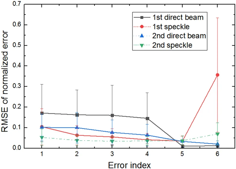
Fig.8 RMSEs of different normalized errors between estimations,for the model trained on the simulation data as first guess and ground truth.Error indices are the same as in Fig.7

To explore the training process of the neural network model for the estimation of the misalignment errors of KB mirrors more clearly, we drew feature maps of the networks extracted from one detected image and show them in Fig.9.The first convolution layer was responsible for extracting related information from the input image and standardizing the format of the feature images.It mainly focused on highintensity loci.The first layer of ResNet extracted texturerelated information from the image and distinguished the speckles surrounding the center beam image and different texture patterns in the beam image.The second layer further extracted texture features, while the third layer summarized the features.As shown in Fig.9d, both localized and global features were present in the feature maps of the third layer.The last convolution layer of ResNet extracted highly abstract information with a large field of view.Instead of fine textured features, this layer yielded coarse-grained structural features.

The saliency map of the network attention is shown in Fig.10.The network extracted information from both the detected beam and speckles surrounding the beam.It also successfully avoided positions with saturated intensity at the lower and right edges of the beam that did not contain any information.Using this technique with a well-trained neural network that can make accurate estimations, we can trace which features were captured by the network and how the features were processed to obtain the result, which can help us verify whether the network learned the mechanics correctly rather than simply fitting data by some tricky means.By careful examination and analysis of the feature processing and attention capabilities of the model, we can understand the structural relationship of input images to target values and may find directions to explain the estimation process and establish the relationship between the detected phenomena and underlying factors.

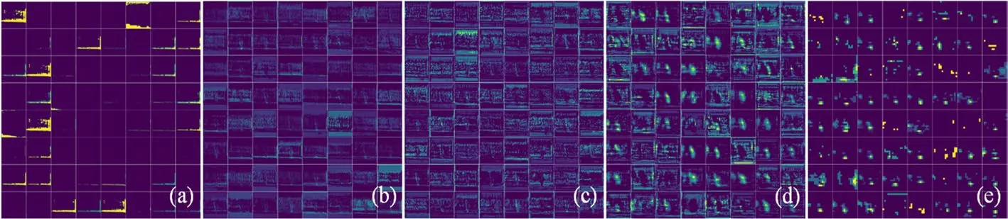
Fig.9 (Color online) Feature maps of convolution layers of misalignment error estimation models trained on the experimental data.From a to e shown are feature maps from the first convolution layer, layer 1 of ResNet50, layer 2 of ResNet50, layer 3 of ResNet50, and layer 4 (the last layer) of ResNet50; each picture contains 64 feature maps.For layers containing more than 64 feature maps, only the first 64 feature maps are shown

Fig.10 (Color online) Saliency maps for the misalignment error estimation models trained on the experimental data.a Input image and b the saliency map generated for this input image

5 Conclusion

A machine learning-based method was presented for estimating the KB mirror alignment error.Direct-beam and speckle-modulated images were captured by a detector for a CNN to estimate the alignment errors.In this study, we used simulations to predict the different performances of detected images under different alignment errors and scatterer conditions and generated training data for deep learning.We verified this method experimentally and estimated the effect of the beam quality.Both experiments exhibited good estimation accuracy, which proved the repeatability of this method.The results demonstrate the applicability of the proposed method.

The proposed method can provide fast and relatively accurate alignment error estimation based on a singleexposure experiment, even under noisy beam conditions.Compared with the existing methods, the proposed method is much faster and more robust and can make estimations with the best normalized RMSE accuracy of 4% on average taking 0.13 s.Similar approaches can be applied to other machine learning-based beam diagnosis problems.By combining simulations and multiple experiments with related visualization technology, we aimed to provide a reliable, trustworthy, and traceable deep learning-based optical metrology approach.However, the error estimation of the network relies heavily on the layout of the beamline and calibration accuracy.The estimation becomes inaccurate if the beamline is modified because the network cannot learn the intrinsic relationship between the alignment error and beam propagation.In addition, different networks for different beamline layouts require large amounts of data and time to train.In future studies, we will optimize the light source model and elucidate the role of mirror figure errors in the beam propagation.A more accurate model will significantly improve the accuracy of the proposed method.For further applications, the robustness, reliability,and generalization of machine learning methods in optical tasks should be improved.This framework can be applied to a wide range of optical imaging systems involving the alignment of optical elements.With the improvement of the analytical ability of neural networks and the development of adaptive optical techniques, we are hopeful that this method will eliminate the dependency on specific scenarios and will enable learning from a generalized beam-generating scheme,avoiding repetitive training on different optical layouts while providing better estimations.This will be helpful for advancing toward a fully intelligent beamline control.

AcknowledgementsThe authors thank Ya-Nan Fu and Guo-Hao Du from Beamline 13HB for their assistance in testing the focusing system and verifying the method described in this paper.

Author contributionsAll authors contributed to the study conception and design.Material preparation, data collection, and analysis were performed by Na-Xi Tian, Hui Jiang, Shuai Yan, Dong-Xu Liang,Ai-Guo Li, Jun Hu, and Jia-Nan Xie.The first draft of the manuscript was written by Jia-Nan Xie, Hui Jiang, Ai-Guo Li, and Jun Hu, and all authors commented on previous versions of the manuscript.All authors read and approved the final manuscript.

Data availabilityThe data that support the findings of this study are openly available in Science Data Bank at https:// www.doi.org/ 10.57760/ scien cedb.j00186.00138 and https:// cstr.cn/ 31253.11.scien cedb.j00186.00138