Variability of Young Stellar Objects in the Perseus Molecular Cloud
2023-09-03XiaoLongWangMinFangGregoryHerczegYuGaoHaiJunTianXingYuZhouHongXinZhangandXuePengChen
Xiao-Long Wang,Min Fang,Gregory J.Herczeg,Yu Gao,Hai-Jun Tian,Xing-Yu Zhou,Hong-Xin Zhang,and Xue-Peng Chen
1 Purple Mountain Observatory,Chinese Academy of Sciences,Nanjing 210023,China;xlwang@pmo.ac.cn,mfang@pmo.ac.cn
2 University of Chinese Academy of Sciences,Beijing 100049,China
3 School of Astronomy and Space Science,University of Science and Technology of China,Hefei 230026,China
4 Kavli Institute for Astronomy and Astrophysics,Peking University,Beijing 100871,China
5 Department of Astronomy,Peking University,Beijing 100871,China
6 Department of Astronomy,Xiamen University,Xiamen 361005,China
7 School of Science,Hangzhou Dianzi University,Hangzhou 310018,China
8 Key Laboratory for Research in Galaxies and Cosmology,Department of Astronomy,University of Science and Technology of China,Hefei 230026,China
Abstract We present an analysis of 288 young stellar objects(YSOs)in the Perseus molecular cloud that have well defined g and r-band lightcurves from the Zwicky Transient Facility.Of the 288 YSOs,238 sources (83% of our working sample)are identified as variables based on the normalized peak-to-peak variability metric,with variability fraction of 92% for stars with disks and 77% for the diskless populations.These variables are classified into different categories using the quasiperiodicity (Q) and flux asymmetry (M) metrics.Fifty-three variables are classified as strictly periodic objects that are well phased and can be attributed to spot modulated stellar rotation.We also identify 22 bursters and 25 dippers,which can be attributed to accretion burst and variable extinction,respectively.YSOs with disks tend to have asymmetric and non-repeatable lightcurves,while the YSOs without disks tend to have(quasi)periodic lightcurves.The periodic variables have the steepest change in g versus g-r,while bursters have much flatter changes than dippers in g versus g-r.Periodic and quasiperiodic variables display the lowest variability amplitude.Simple models suggest that the variability amplitudes of periodic variables correspond to changes of the spot coverage of 30%–40%,burster variables are attributed to accretion luminosity changes in the range of Lacc/L★=0.1–0.3,and dippers are due to variable extinction with AV changes in the range of 0.5–1.3 mag.
Key words: stars: variables: general–stars: late-type–stars: emission-line–Be–(stars:) starspots–accretion–accretion disks
1.Introduction
Photometric variability was one of the original defining characteristics of young stellar objects(YSOs),even before the sources were known to be young (Joy 1945,1946).Different components of the YSO system (star+disk) dominate different part of the spectral energy distribution (SED) of the YSO,so monitoring at different wavelength probes the physical processes in different parts of the system (Venuti et al.2021;Fischer et al.2022).Optical monitoring is powerful for understanding the stellar rotation of spots of the stellar photosphere,accretion from the disk onto the star,and dust obscuration (e.g.,Cody et al.2022;Hillenbrand et al.2022).Monitoring in the near-and mid-infrared bands has been used to study the warm dust in the disk,including the inner rim(e.g.,Skrutskie et al.1996;Carpenter et al.2001;Makidon et al.2004;Morales-Calderón et al.2011;Rebull et al.2014;Park et al.2021).These studies reveal higher fraction of variables for YSOs than for main-sequence stars,and that disked YSOs are more variable than diskless YSOs.
Time series photometry have revealed a diversity of lightcurve shapes,including dipping stars exhibiting episodic or quasiperiodic fading events (e.g.,Alencar et al.2010;Bodman et al.2017),bursting stars exhibiting discrete brightening events (e.g.,Stauffer et al.2014),and periodic variables displaying sinusoidal-like lightcurves.Many lightcurves have complicated shapes,with more than one potential phenomenon shaping the changes on many timescales.Cody et al.(2014) defined the flux asymmetry (M) and quasiperiodicity (Q) metrics to classify regularly sampled lightcurves from space-based observations into 7 categories: periodic,dipping (including quasiperiodic dipper and aperiodic dipper),bursts,quasi-periodic,stochastic,and long-timescale.There are also other schemes classifying YSOs into different variability categories(see Section 5.1 of Cody et al.2014,for a review).In this work,we use the classification scheme of Cody et al.(2014) to separate the lightcurves into different categories.
Various mechanisms are responsible for the diversity of lightcurve shapes.Strictly periodic objects are attributed to rotational modulation due to the presence of star spots on the stellar surface,rotating into and out of view.The variability of dipping stars (both quasiperiodic and aperiodic dippers) is commonly explained as stemming from variable extinction due to time-dependent occultation by circumstellar material (Alencar et al.2010;Morales-Calderón et al.2011;Turner et al.2014;Ansdell et al.2016).Burst variables tend to display strong Hα emission and red infrared colors (Cody &Hillenbrand 2018),and their variability are related to accretion bursts(Stauffer et al.2014).Stochastic lightcurves are likely to arise from continuously stochastic accretion behavior producing transient hot spots (Stauffer et al.2016).Quasiperiodic behavior is generally interpreted as purely spot behavior on top of longer timescale aperiodic changes or a single variability behavior varies from cycle to cycle (Cody et al.2014).The most probable mechanisms driving long timescale variability include variable extinction and variable accretion activity(Parks et al.2014).
Time series photometry from the Zwicky Transient Facility(ZTF;Kulkarni 2018) has been used to study large samples of periodic variables (Chen et al.2020),as well as to investigate the variability behavior in YSOs (Hillenbrand et al.2022,hereafter H22).In this paper,we analyze the variability properties of YSOs in the Perseus molecular cloud,using the time series photometry from the ZTF.The data set and the sample are described in Section 2.The properties of the targets are determined in Section 3.In Section 4 we present the analyses of the lightcurves,the variability properties of our sample,and the CMD pattern.A discussion relating CMD patterns to simple models is presented in Section 5.We give our summary in Section 6.
2.Data Set and Target Selection
2.1.YSO Catalog
In our previous work (Wang et al.2022),we collected a sample of 805 previously known members from various literature (i.e.,Luhman et al.2016;Esplin &Luhman 2017;Kounkel et al.2019;Luhman&Hapich 2020)and identified 51 new members based on Gaia astrometry (Gaia Collaboration et al.2021;Fabricius et al.2021;Riello et al.2021) and LAMOST spectroscopy(Luo et al.2022),resulting in a total of 856 well confirmed members in the Perseus molecular cloud.This sample of 856 members constitutes our initial YSO sample.The spatial distribution of the initial sample as well as our working sample (discussed below) are displayed in Figure 1.
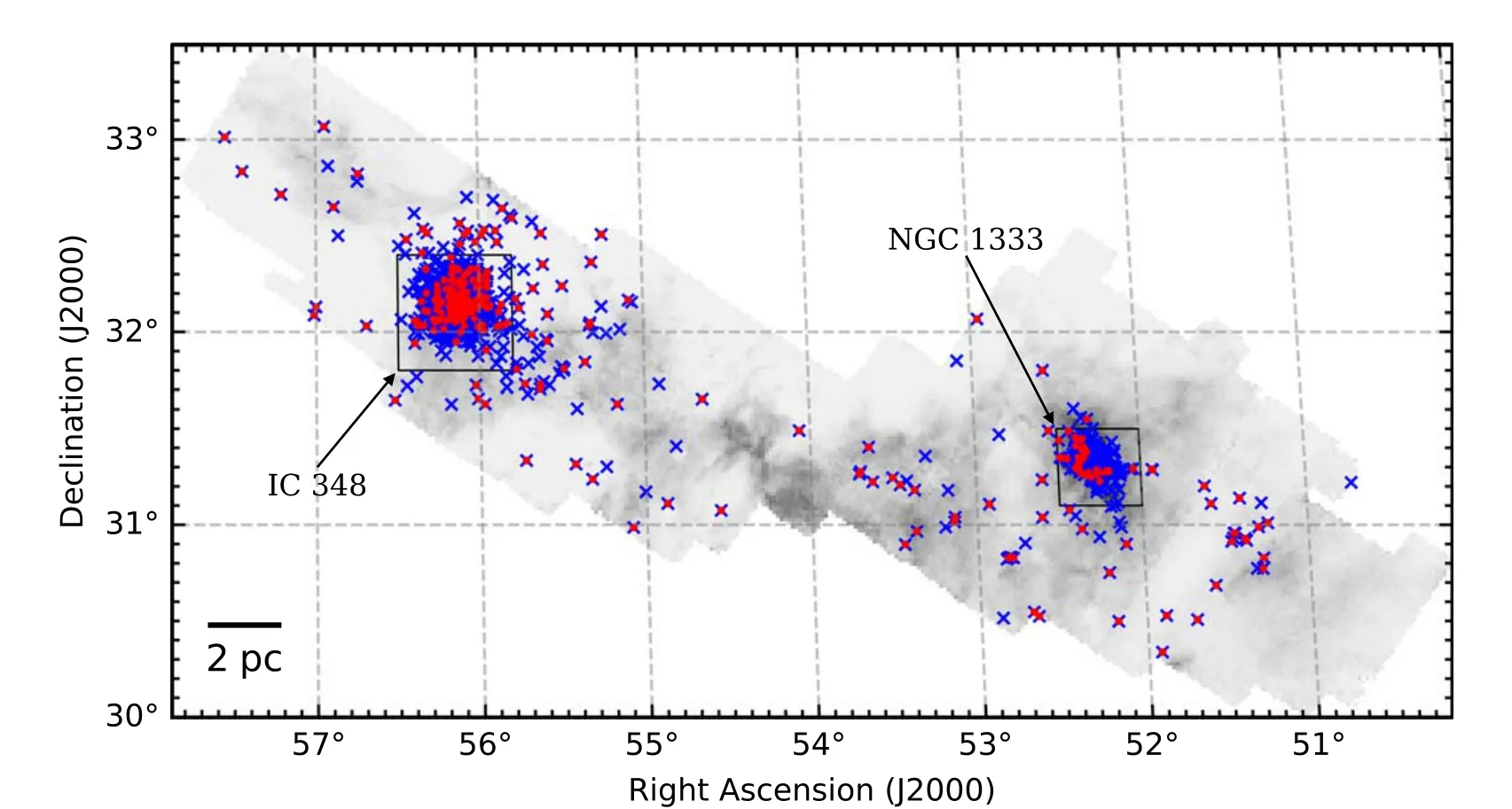
Figure 1.Spatial distribution of the initial YSO sample (blue crosses) overlaid on the FCRAO 12CO J=1 →0 integrated intensity map (Ridge et al.2006).Additional red points mark the 288 sources in our working sample.The two rectangles mark the two young clusters IC 348 and NGC 1333.The scale bar on the lower left shows a size of 2 pc at a distance of 300 pc.
2.2.ZTF Photometry
The ZTF (Kulkarni 2018) is a time-domain photometric survey currently in progress.It uses a 47 deg2camera consisting of 16 individual CCDs each 6k×6k covering the full focal plane of the Palomar 48 inch (P48) Schmidt Telescope at Palomar Observatory (Masci et al.2019).In this paper,we analyze data from the 13th public ZTF data release(ZTF DR139https://irsa.ipac.caltech.edu/data/ZTF/docs/releases/dr13/ztf_release_notes_dr13.pdf),which corresponds to more than four years of data taken between 2018 March 17 and 2022 July 8 (58194 ≤MJD ≤59768).The photometry is provided in theg,randibands,with a uniform exposure time of 30 s in the public survey and is calibrated to the PanSTARRS photometry and reported in AB magnitude.The ZTF DR13 contains about 4.4 billion lightcurves in theg,roribands,with more than half of them have ≥20 epochs of observations.Ther-band have the most number of lightcurves.
Searching the ZTF archive,we extractg-band lightcurves for 466 members andr-band lightcurves for 577 members of the Perseus molecular cloud.In this work,we will focus our analysis on the ZTFgandr-band lightcurves only,since noiband lightcurve is available for our targets.We ignore observations with catflags=32768 that are affected by clouds or contaminated by the moon.For our analysis,we restrict ourselves to sources with mean magnitudes brighter than 20.8 and 20.6 in thegandr-band respectively10These magnitudes correspond to the median 5σ sensitivity in 30 s of g and r-bands,respectively (Bellm et al.2019;Masci et al.2019).,over the entire time series.Following the procedure in H22,we further remove observations taken on MJD days 58786,58787,58788,58789 and 58805,that are part of the ZTF high-cadence experiments (Kupfer et al.2021) and affect the period search.To alleviate the impact from potential outlier measurements in the lightcurves,we remove measurements 5σ away from the median magnitude of the corresponding lightcurve.In some cases,an additional one to three points are found to be nonphysically discrepant and are removed.Finally,only lightcurves (5σ clipped) with more than 30 measurements are considered for further analysis.Several sources which are located closely are not resolved by the ZTF are removed.In the current work,we only focus on G to M type members.Our final sample contains 288 sources with bothg-andr-band lightcurves.
2.3.LAMOST Spectroscopy
The Large Sky Area Multi-Object Fiber Spectroscopic Telescope (LAMOST),also called the Guo Shoujing Telescope,is a quasi-meridian reflecting Schmidt telescope located at Xinglong Observatory Station in Hebei province,China.The telescope has an effective aperture of~4 m and a field of view of 5° in diameter.The telescope is equipped with 16 spectrographs and 4000 fibers,each spectrograph has a resolving power ofR≈180011The spectrographs have been upgraded to support median resolution observations with R ≈7500 since 2018 (Liu et al.2020).,and the wavelength coverage is 3700-9100 Å(Cui et al.2012;Zhao et al.2012;Liu et al.2015;Luo et al.2015).
Cross matching our working sample with the data release 9 of the LAMOST survey (LAMOST DR912http://www.lamost.org/dr9/),we obtain LAMOST spectra for 174 members in our working sample.There are 151 sources showing prominent Hα emission lines in their LAMOST spectra.The accretion properties of these Hα emitters are studied in Section 3.3.
3.Target Properties
3.1.Stellar Masses and Ages
Spectral types and extinction corrections have been provided for the full YSO sample (Luhman et al.2016;Esplin &Luhman 2017;Kounkel et al.2019;Luhman &Hapich 2020;Wang et al.2022).We use the same methods as described in Wang et al.(2022) to convert spectral types and observedJmagnitudes to effective temperatures and bolometric luminosities,respectively,and then to construct the Hertzsprung–Russell (H-R) diagram (Figure 2).Stellar masses and ages are estimated from their locations on the H-R diagram for individual sources using the PARSEC stellar model (Bressan et al.2012).In Figure 3,we display the distributions of stellar ages and stellar masses.Though they span a large range of age,most objects in our working sample have ages between 1 and 10 Myr,with median age of 3.8 Myr.More than 90% of the objects in our working sample are less massive than 1M⊙,and the median mass is 0.5M⊙.

Figure 2.H-R diagram of the objects in our working sample.Overlaid are the isochrones (red solid lines) and mass tracks (blue dashed lines) with solar metallicity from the PARSEC stellar model (Bressan et al.2012),with their corresponding ages and masses indicated.The red dotted line is the stellar birth line.

Figure 3.Histograms showing the distribution of stellar ages (left) and stellar masses (right) for the objects in our working sample.These values are estimated using the PARSEC stellar model (Bressan et al.2012) without correcting the contribution from spots.
3.2.Disk Classification
Most of the objects in the full YSO sample have disk classifications based mainly onSpitzerphotometry (Dunham et al.2015;Luhman et al.2016;Kounkel et al.2019).We reclassified six of objects as disks based on their very redKS-W2 colors (marked with blue squares in Figure 4).One additional object is also reclassified as a disk based on its excess emission atW4 andMP1 bands (marked with green square in Figure 4).Forty objects in our working sample with no disk classifications from the literature are classified here based on their locations on theKS-W2 versusH-KScolor–color diagram (Figure 4).Objects withKS-W2 colors redder than 0.98×(H-KS)+0.22 are classified as disks and bluer as diskless(Wang et al.2022).The dividing line separating disks from diskless YSOs is constructed as follows.The locus of objects having disk classifications from literature is compared to the dwarf locus from Pecaut &Mamajek (2013) and reddening vector from Wang &Chen (2019).Visually inspecting the color–color plot indicates that vertically shifting the upper border of the dwarf locus due to reddening redward of 0.15 mag can separate disked YSOs from diskless ones fairly well.Five of these 40 objects are classified as disks,and the remaining as diskless ones.We also note that several sources classified as disks in the literature are located at the diskless boundary in Figure 4,because their infrared excess is seen only at wavelengths longer thanW2.

Figure 4.Infrared color–color plot for objects in our working sample.The solid circles and plus signs represent disked and diskless YSOs,respectively.Objects classified by us are highlighted as red.Additional blue and green squares mark sources that are classified as diskless in the literature.The solid curve is the locus of dwarfs from Pecaut &Mamajek (2013),and the dashed lines correspond to the extinction law from Wang &Chen (2019),enclosing the color space of dwarfs due to reddening.The dashed–dotted line is the dividing line that we use to separate disked YSOs from diskless ones(see Section 3.2 for detail).
Our working sample comprises of 109 disk objects and 179 diskless objects.The disk fraction of objects in our working sample is 38%,slightly lower than that of the initial sample(46%).This discrepancy is mainly due to that our working sample is constructed based on the ZTF photometry,which may be biased against low mass or embedded objects and stars with edge-on disks.We note that the disked and diskless objects in our working sample share similar mass ranges,and the majority of both samples are less massive than 1M⊙.The KS-test indicates that the two samples are indistinguishable in terms of spectral types (p=7%).
3.3.Accretion Properties
Accreting YSOs are generally characterized by strong and broad emission lines in their optical to near-infrared spectra(Hartmann et al.1994;Muzerolle et al.1998a,1998b).Correlations between emission line properties and accretion have been established both theoretically and observationally(e.g.,Muzerolle et al.1998a;Natta et al.2004;Fang et al.2009).Hα is one of the strongest emission lines in classical T Tauri stars (CTTSs) and has been widely used as an indicator of accretion activity (Muzerolle et al.2003;White &Basri 2003;Natta et al.2004;Fang et al.2009,2013).
In this section,we use the Hα emission lines to study the accretion activities for a sub-sample of our working sample.We use the equivalent widths of Hα emission lines (EWHα) to distinguish between CTTSs and weak-line T Tauri stars(WTTSs) for the disk population.Since there is no unique EWHαvalue to distinguish all CTTSs from WTTSs,due to the “contrast effect”(Basri &Marcy 1995)and line optical depths(Ingleby et al.2011),we adopt the spectral type dependent thresholding values from Fang et al.(2009) to distinguish between CTTSs and WTTSs,that is an object is classified as CTTS if EWHα≥3 Å for K0-K3 stars,EWHα≥5 Å for K4 stars,EWHα≥7 Å for K5-K7 stars,EWHα≥9 Å for M0-M1 stars,EWHα≥11 Å for M2 stars,EWHα≥15 Å for M3-M4 stars,EWHα≥18 Å for M5-M6 stars,EWHα≥20 Å for M7-M8 stars.We further refine the classification by assigning the diskless objects as WTTSs.Forty sources are classified as CTTSs,and 134 sources are classified as WTTSs.Of the WTTSs,86% (116/134) are diskless objects.
4.Lightcurve Analysis
Most objects in our working sample have 200–500 observations during the~4 yr ZTF data stream.Since therband photometry is much better than theg-band and the cadence is generally higher in ther-band than in theg-band,our analysis of the lightcurves in this section is mainly based on ther-band photometry.Theg-band photometry is only used in analyzing the CMD pattern and when mentioned specifically.
4.1.Variability Search
We use the normalized peak-to-peak variability metric(Sokolovsky et al.2017)
to measure variability amplitude for objects in our working sample,wheremiis a magnitude measurement and σiis the corresponding measurement uncertainty.The maximum and the minimum are determined from the full lightcurve.The normalized peak-to-peak variability is a sensitive variability indicator (Sokolovsky et al.2017) since we have removed potential outliers from each lightcurve (see Section 2.2).
Following H22,we consider an object variable if its ν metric is greater than the 15th percentile of ν as a function of meanrmagnitude (Figure 5).As pointed out in H22,although this is not a rigorously justified cutoff,this cut ensures that we select the fractionally larger amplitude objects as variables at each brightness level.We select 238 (83% of our working sample)objects as variables based on the ν metric.

Figure 5.Normalized peak-to-peak variability metric ν as a function of mean r magnitude for our working sample.Disked and diskless objects are indicated with red circles and blue pluses,respectively.The black solid line is the 15th percentile line,i.e.,the boundary line we use to distinguish between variables and non-variables.The red and blue solid lines mark the median trends for disk and diskless populations,respectively.
92%of the disk population and 77%of the diskless population are variables.The variability fraction of the disk population is much higher than that of the diskless population,as can be more evidently seen in Figure 5.In addition,the ν metrics are typically 1–3 times larger for disk population than for diskless population(as indicated with red and blue solid lines in Figure 5).
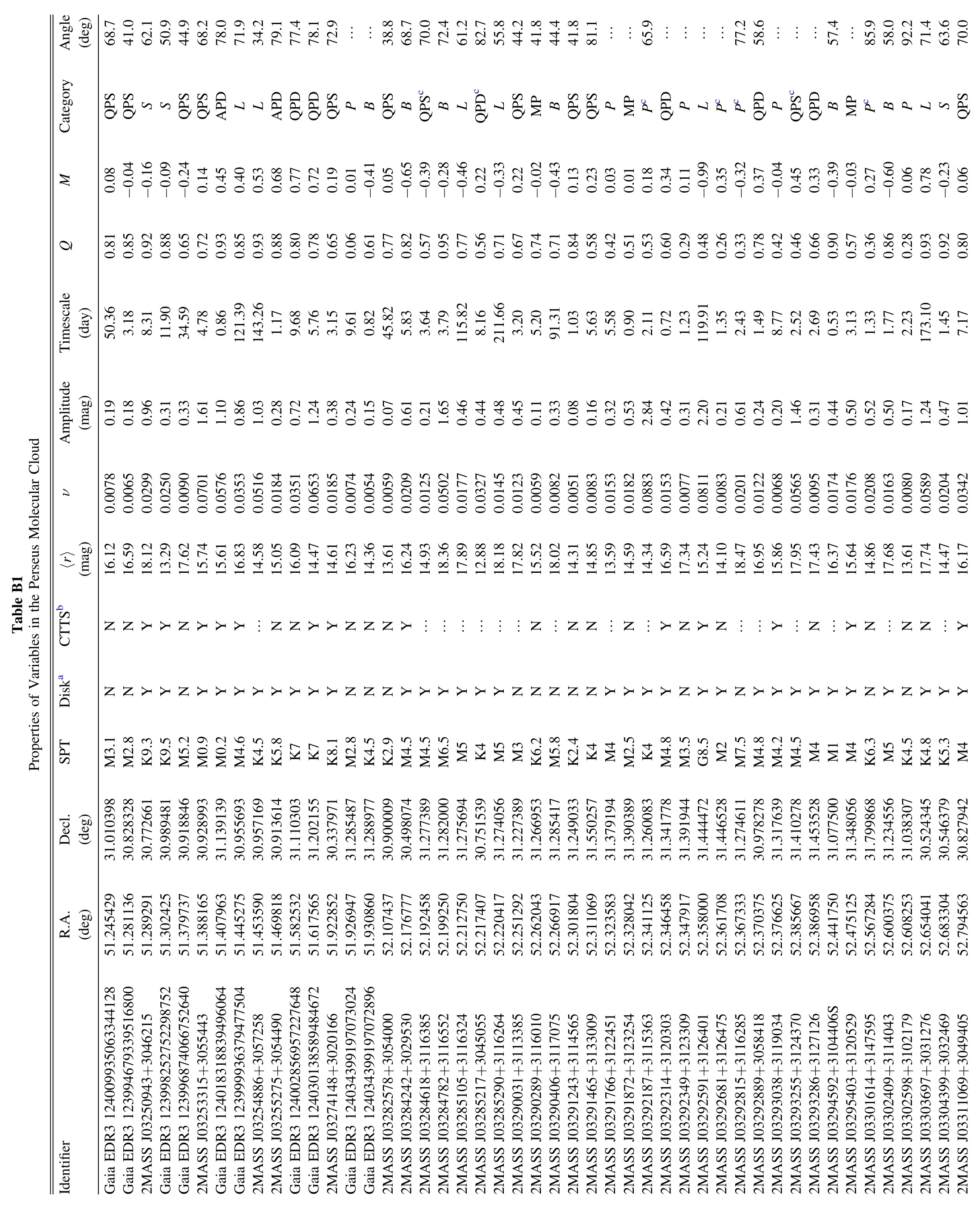
The properties of the 238 variables are listed in the table in Appendix B.The variability amplitude listed in the table is calculated as the difference between the 5th and 95th percentile magnitudes.
4.2.Period Search
We use the Astropy (Astropy Collaboration et al.2013,2018)implementation of the Lomb-Scargle periodogram(Lomb 1976;Scargle 1982;VanderPlas &Ivezić 2015;VanderPlas 2018) to compute the periodogram for each variable and search for periods between a minimum period of 0.5 days and a maximum period of 250 days.Periods between 0.5-0.51,0.98-1.02,1.96-2.04,and 26-30 days are flagged for further analysis to avoid the most common aliases associated with the solar and sidereal days,as well as the lunar cycle (Rodriguez et al.2017;Ansdell et al.2018;Hillenbrand et al.2022).We also reject periods with half or double multiples that fail at least one of the aforementioned alias checks to account for additional potential aliases.In most cases,the period is searched using ther-band lightcurve,except for cases where theg-band lightcurve is better phased.
We then use the find_peaks13https://docs.scipy.org/doc/scipy/reference/generated/scipy.signal.find_peaks.htmlfunction from the PYTHON package scipy (Virtanen et al.2020) to search for power peaks in the periodogram.Only peaks higher than the 1% false alarm level14Since the true probability distribution for the largest peak cannot be determined analytically,we estimate the false alarm probability approximately using the approach of Baluev (2008).are considered significant,and are retained for further analysis.If there are no peaks more significant than the 1% false alarm probability,we take the period corresponding to the maximum power of the periodogram as estimates of the variability timescales.In most cases the peak with the maximum power is adopted as the real period,but there are cases where the peak with slightly lower power is adopted as the real for better interpreting the beat patterns and improving the phase dispersion minimization(i.e.,with smallerQvalues determined in the next section).
For sources with multiple peaks in the periodogram,the frequencies of the peaks are checked for possible alias and beats following the proposals in VanderPlas(2018).The source is labeled as multiperiodic if there are peaks with frequencies that are not alias or beats of the adopted real period.Based on our visual inspection,only the first four highest peaks are checked for sources with more than four peaks in their periodograms.
The distribution of the periods or timescales are displayed in Figure 6.Our variable sample has a relatively flat distribution,extending to more than 200 days.For the periodic objects,our sample is double peaked with a tail toward longer periods.The two peaks at around 1.5 days and one week are consistent with the populations of fast and slow rotators,respectively(Gallet&Bouvier 2013).

Figure 6.Histograms showing the distribution of periods or timescales of the periodogram peaks.The left panel shows all timescales,and the right panel shows only sources classified as periodic variables.
We compare our periods with that from literature (e.g.,Rebull et al.2015;Fritzewski et al.2016)in Figure 7.In most cases,our periods are consistent with that from literature.The largest discrepancy is found for objects we classified as quasiperiodic,for which we found periods that are aliases of the literature periods with the 1 day sampling.

Figure 7.Comparison of periods between our work and previous literature for sources that we classified as periodic (filled symbols) or quasiperiodic symmetry (open symbols).Circles are periods from Fritzewski et al.(2016)and squares are periods from Rebull et al.(2015).Different lines indicate the different harmonics and the alias with the~1 day sampling as shown in the legend.The x in the legend represents our periods and y is literature periods.
4.3.Lightcurve Classification
We classify our lightcurves into different types based on two statistics quantifying quasiperiodicity (Q) and flux asymmetry(M),first developed by Cody et al.(2014) based on regularly sampled time series from space-based platforms and further refined by Cody &Hillenbrand (2018).TheQandMmetrics are defined as follows,
where σmis the scatter of the original lightcurve,σresdis the scatter of the residual lightcurve after subtracting the smoothed dominant periodic signal,σphotis taken as the mean photometric error of all observations in an object’s lightcurve,scaled by a factor of 1.25 to account for an initial compression ofQvalues (H22),mmedis the median magnitude of the lightcurve,and〈m10%〉 is the mean magnitude of the top and bottom 10% measurements.The reader is referred to H22 for more details on theQandMmetrics.In most cases,theQandMmetrics are calculated for each variable using ther-band lightcurve data.For several cases,the period is determined for theg-band lightcurve only,and theg-band lightcurve is used to determine these statistics.The variables in our working sample are classified into nine categories,based on their locations in theQ-Mplane (Figure 8) and additional visual inspection.
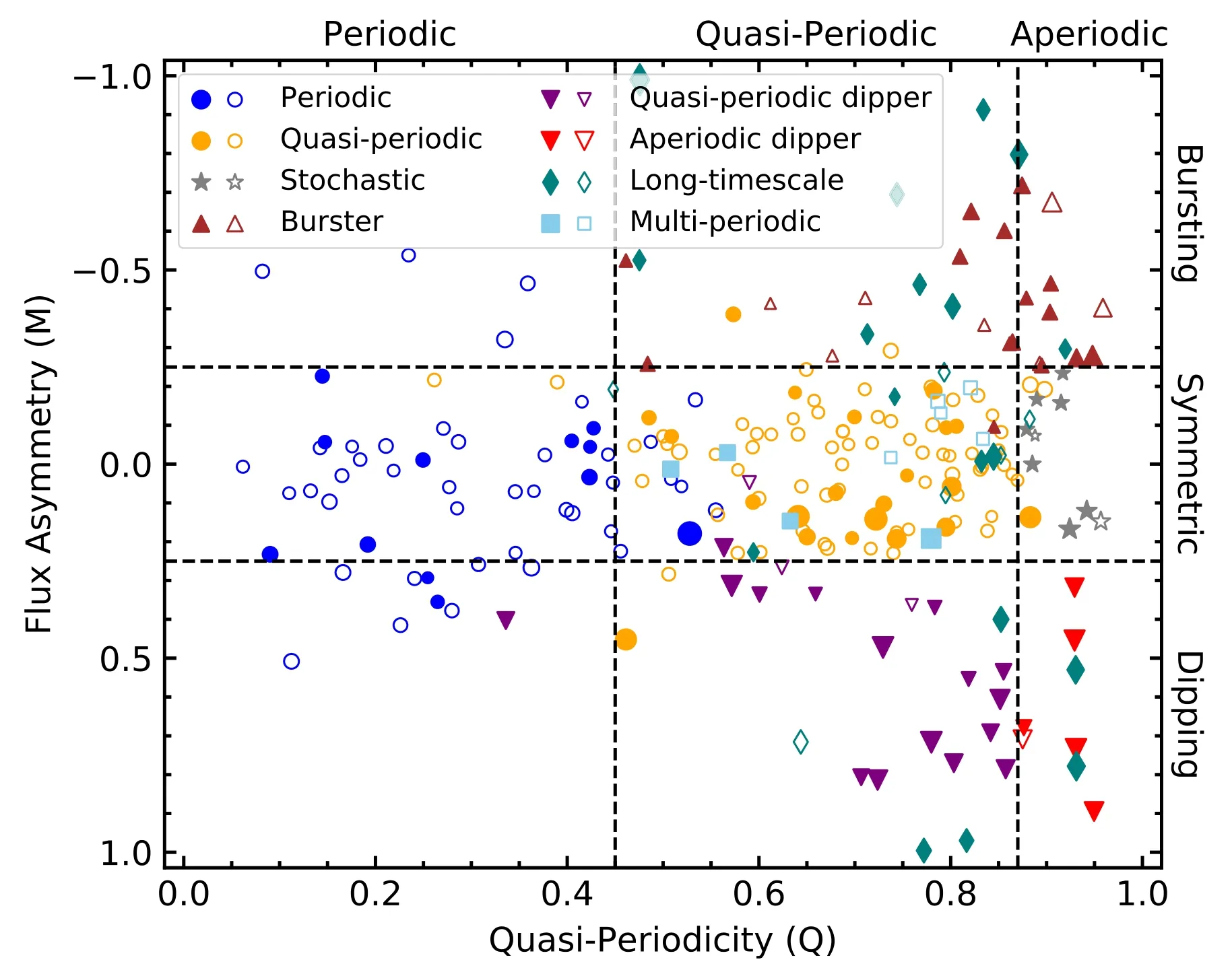
Figure 8.Quasiperiodicity (Q) vs.flux asymmetry (M) for our sample of variables,color coded by lightcurve morphological types.The sizes of the points are proportional to the square root of the normalized peak-to-peak variability metric ν.Disked objects are indicated with solid symbols and diskless objects are marked with open symbols.Note that unclassifiable variables are not included in this plot,since they fall off the viewing range of the plot.
Since the time series data analyzed here is from the same instrument as in H22,we adopt the same boundary values ofQandMmetrics as H22.The boundary values used to classify the lightcurves into different variability categories are summarized and listed in Table 1.In addition to the seven categories listed in Table 1,we classify objects with variability timescales larger than 100 day as long timescale (L) variables,and objects having more than one periods are classified as multi-periodic(MP) variables.All of the lightcurves and corresponding periodograms are visually inspected.In most cases,theQandMclassifications are consistent with our visual inspection.For 40 cases(labeled in Table B1),we adjust their type to favor our visual classification.We note that the original classification scheme does not involve theQ-Mplane with 0 <Q<0.45 andM>0.25.About 10 of these cases have (Q,M) values in this region,and these sources are classified as periodic variables based on their well phased lightcurves.Other adjustments mainly occur around the boundaries,and the most common adjustment is from quasiperiodic symmetric category to periodic type for seven objects due to their well-phased lightcurves and their quite clean periodograms.These adjustment does not affect our statistics significantly.We should mention that both the photometric precision and the cadence will affect the measurement of theQmetric,and thus the classification of the lightcurve morphology.The readers are referred to H22 for a discussion on these effects (see their Appendix C).
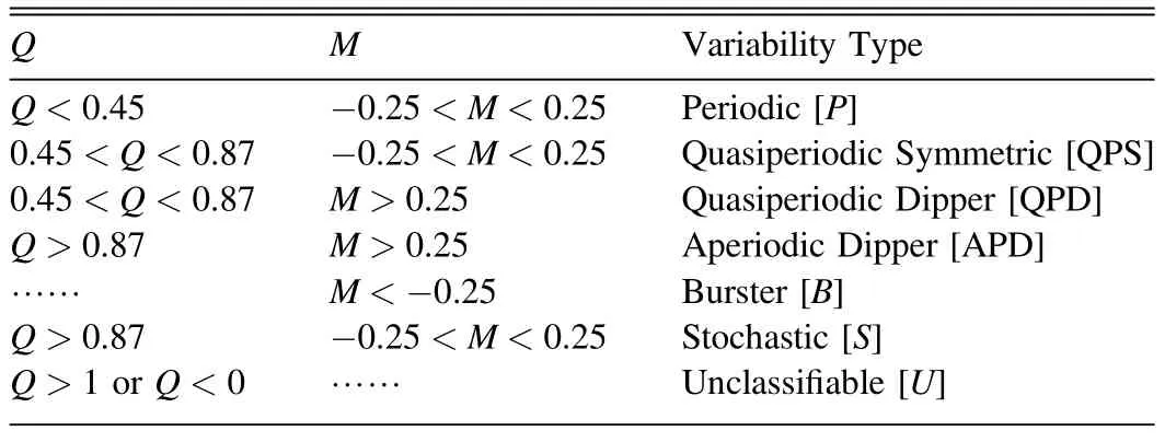
Table 1Criteria used to Classify the Lightcurves into Different Variability Categories
The numbers of different lightcurve morphologies are listed in Table 2.The dominant lightcurve morphology in our variable sample is quasiperiodic symmetric.For the disk population,dipper (both quasiperiodic dippers and aperiodic dippers),burster,stochastic and long timescale categories are also common.We performed two-dimensional Kolmogorov–Smirnov (KS) test (Peacock 1983)15We used the 2D KS-test PYTHON implementation ndtest available at https://github.com/syrte/ndtest.to compare the 2D parameter space (Q,M) for disk and diskless populations.We foundp-value of 2×10⁻⁴corresponding to the null-hypothesis that disk and diskless populations occupy the same (Q,M)space.The disk population is dominated by asymmetric and non-repeatable lightcurves,while the diskless population is dominated by symmetric and repeatable lightcurves.There are 11 diskless objects classified as bursters or dippers.Visually inspecting their lightcurves indicates that they have variability amplitudes comparable to the measurement uncertainties or theirMmetrics are affected by several photometric measurements,which makes their classifications unreliable.As pointed out in Section 3.2,the disk and diskless populations in our working sample share similar mass ranges and spectral type distributions.In addition,we do not find any trends of variability properties as functions of stellar masses or spectral types.Considering these issues together,the differences of the variability patterns of the two populations are dominated by the presence or absence of disks.

Table 2Distribution of Lightcurve Morphological Category for Objects in our Variable Sample
The EWHαvalues are displayed as a function of spectral type and lightcurve morphological category in Figure 9 for a subsample of 146 variables having LAMOST spectra.In the figure,nearly all sources in the burster (brown upward triangles) and stochastic (gray star symbols) categories are CTTSs.Half of the dippers and long timescale variables are also CTTSs.More than 85%(90/105)of variables classified as P,QPS,or MP are WTTSs.The numbers of different lightcurve types in this sub-sample are listed in Table 2.These are consistent with the results on the different properties of the disked or diskless variables discussed above.
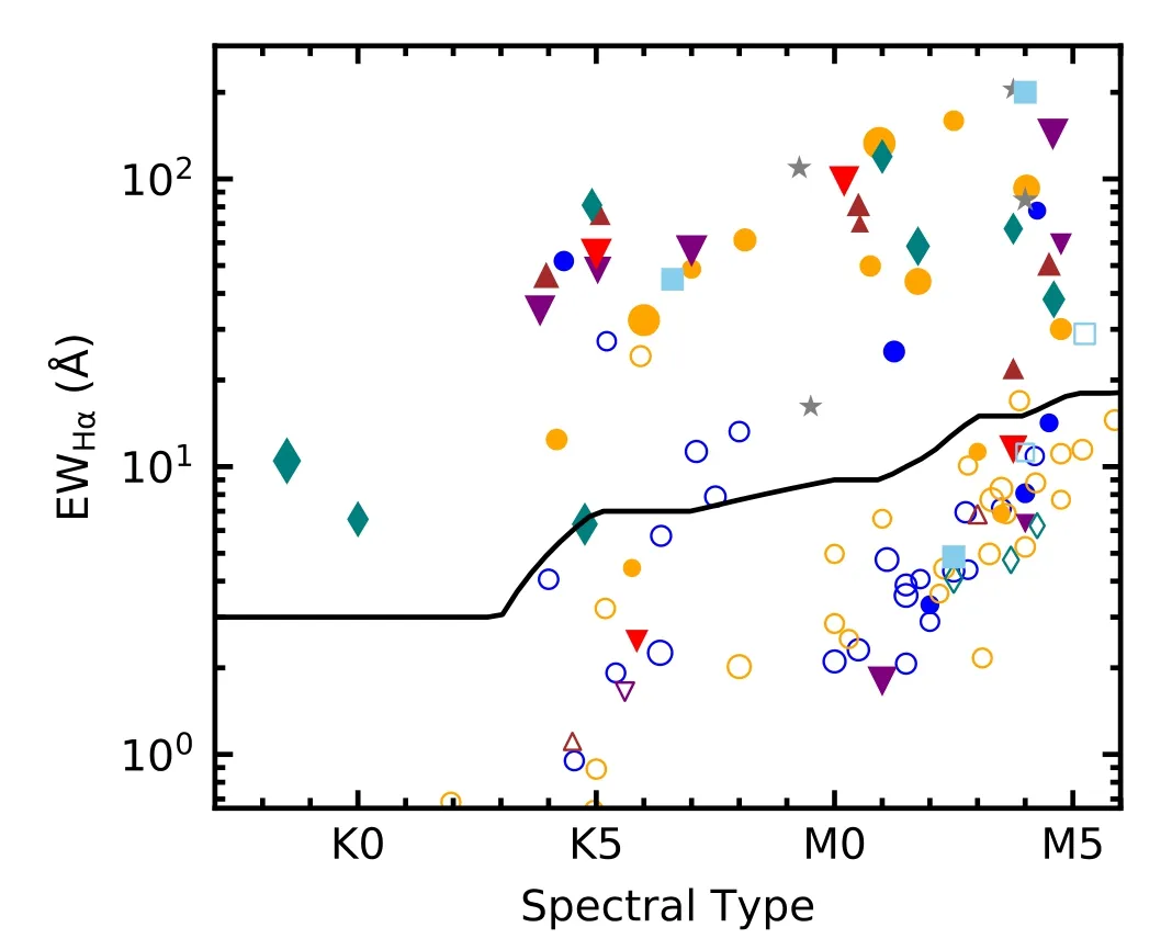
Figure 9.Equivalent width of Hα emission line as a function of spectral type.The symbols are the same as in Figure 8.The solid line is the dividing line separating CTTSs from WTTSs (Fang et al.2009).
4.4.CMD Analysis
There are many different physical mechanisms that can drive the photometric variability observed in young stars (see H22 for a summary of the mechanisms related to different lightcurve morphologies).Color time series data is a powerful tool in distinguishing these physical mechanisms.Our working sample is constructed to have bothgandr-band lightcurves,so it is possible for us to analyzeg-rcolor times series data,besidesgorr-band lightcurves.
Since the ZTFgandr-band observations are not simultaneous,with time steps of a few hours up to a few days,we construct the CMDs with the following two methods.
The first method (Method 1) is the same as that in H22.For each source,ther-band lightcurve is trimmed into the correspondingg-band time span.For each time point in the trimmedr-band lightcurve,we search theg-band lightcurve for paired observations with one just before this time and another after this time,we then linearly interpolate the pairedg-band observations to this time point and to estimate theg-rcolors,if the time interval of the pairedg-band observations is less than 3 days.The errors of the interpolatedgmagnitudes andg-rcolors are estimated using the PYTHON package uncertainties (Lebigot 2010).
The second method (Method 2) that we developed to construct the CMD is based on the phase-folded lightcurves and applied to only periodic objects in our sample.For periodic objects,both thegandr-band lightcurves are phase-folded at the adopted periods.The median magnitudes,the standard deviations and the number counts are determined for 10 evenly spaced phase bins,for both thegandr-band lightcurves,for each source.The errors of the magnitudes corresponding to each phase bin is estimated as the standard deviation divided by the square root of the number count,of that phase bin.Theg-rcolors are estimated at the same phase,with the errors estimated using the uncertainties package as well.The CMD constructed this way will be designated the phase series CMD in the remaining of the paper.An example of constructing the phase series CMD is displayed in Figure 10.

Figure 10.An example displays constructing the phase series CMD for the source 2MASS J03442812+3216002.(a)The g-band phase-folded lightcurve is displayed as small points with error bars.The blue squares show the median magnitudes in individual phase bins,and the horizontal error bars are the corresponding phase bins.The standard deviations of the median magnitudes are smaller than the symbol size.(b)Similar to(a),but for the r-band data.(c)The phase series CMD is displayed as blue points.The black line is the straight line from the orthogonal regression.The error bar in the lower left displays the typical uncertainty of the data points.The corresponding CMD slope angle is labeled.(d) Similar to (c),but displaying the time series CMD for comparison.

Figure 11.Examples showing the lightcurves (left panels) and corresponding CMDs (right panels) for periodic,burster,quasiperiodic dipper and aperiodic dipper categories.In the left panels,the source name,the flux asymmetry(M),the quasiperiodicity(Q),the period/timescale and the lightcurve classification are labeled for each source.In the right panels,the gray lines are the straight line from the orthogonal regression,and the corresponding CMD slope angles are labeled.

Figure 12.Same as Figure 11,but for quasiperiodic symmetric,stochastic,multi-periodic,long timescale and unclassifiable categories.
For each source in the variable sample,we fit a straight line to its time/phase series CMD using an orthogonal distance regression in the PYTHON package scipy.odr (Virtanen et al.2020),following (Poppenhaeger et al.2015;Hillenbrand et al.2022).This method is chosen to account for the significant and partially correlated errors in both axes.For the CMD constructed using the first method,only the central 95%of the CMD spans ingandg-rare included in the regression,to alleviate the effect of outliers.
The slope angles are defined as the inverse tangent of the best-fitting slopes in thegversusg-rCMDs.The slope angles are expressed in degrees and span from 0°(corresponding to color changes with no associatedg-band variability) to 90°(corresponding tog-band variability with no color changes).To estimate the errors on the best-fitting slope angles,the CMD points are perturbed according to the errors ingmagnitudes andg-rcolors assuming Gaussian errors(this is similar to the perturbation method described in Curran 2014) and the orthogonal distance regression is performed on the perturbed points.This procedure is repeated 1000 times for each source and the errors on the angles are estimated as the standard deviation of the 1000 realizations.Only sources with errors less than 10°are considered for further analysis.This error estimation is slightly different from that in H22,where the errors are estimated using a bootstrap technique.Several examples of the constructed CMDs and corresponding lightcurves are displayed in Figures 11 and 12.
In Figure 13,we display the distribution of CMD slope angle and variability amplitude for different lightcurve morphological categories.Strictly periodic objects show the largest angles,and bursters have much flatter slopes than dippers.Periodic and quasiperiodic sources have the lowest variability amplitudes.In the next section,we demonstrate that the angles of periodic variables are consistent with the spot model,the angles of bursters are consistent with the accretion model,and the angles of dippers are consistent with variable extinction.We also note that stochastic variables have angles in consistent with variable accretion,which may indicate that these sources are ongoing accretion activity as well (as demonstrated in Stauffer et al.2016).All but one of the stochastic variables having LAMOST spectra are accreting stars.

Figure 13.Boxplots showing the distributions of CMD slope angle (left) and variability amplitude (right) for different lightcurve morphological categories.Multiperiodic and unclassifiable categories are not included here.
5.Discussion
In Section 4.3 we classified our variables into different categories and,in Section 4.4 we analyzed the CMD patterns using the orthogonal distance regression technique ong-rversusgCMD.In this section,we will discuss the different CMD patterns of periodic,burster and dipper categories,and relate them with specific mechanisms.
There are 53 (~21% of the variable sample) objects classified as strictly periodic variables,with CMD slope angles determined for 32 of them using Method 1 and Method 2.As shown in the upper left panel of Figure 14,we obtain much larger angles using Method 2 than using Method 1.These periodic variables are generally explained as stellar rotation modulated by star spots on the stellar surface.We model the CMD pattern for a star withTeff=4000 K and a cool spot 500 K cooler than the effective temperature on the stellar surface.The CMD trend arising from the cool spot is nearly vertical,corresponding to colorless variability with associated changes ingmagnitudes and the corresponding slope angle is essentially 90°.Gully-Santiago et al.(2017) also found nearly colorless changes inB-VorV-Rcolors with associated brightness changes in theV-band.Changing the effective temperatures and the temperature contrasts does not alter the angles significantly.

Figure 14.(Left) Histograms showing the distributions of CMD slope angles for periodic,burster and dipper variables from top to bottom,as labeled in the corresponding panels.The gray shaded area display the 1 σ range of the slope angles for non-variables in our sample(see the discussion in Appendix A).The vertical line in each panel corresponds to the angles due to changes in spot coverage,variable accretion and variable extinction,respectively,from top to bottom.The vertical lines in the left top and middle panels are calculated for Teff=4000 K.The blue and red histograms in the left top panel represent the angles determined using Method 1 and Method 2,respectively.(Right) The variability amplitudes observed are compared to that due to changes of spot coverage,variable accretion and variable extinction for periodic,burster and dipper variables,respectively,from top to bottom.The red horizontal line and the shaded area in each panel show the median value and the 1 σ range of the amplitude for the corresponding sample,respectively.The solid and dashed lines in the right top and middle panels correspond to calculations for Teff=4000 K and 3500 K,respectively.
Comparing the slope angles that we determined with this simple model,we find that the angles from Method 2 are more consistent than from Method 1 with the cool spot model.One possible reason could be that the interpolation of theg-band observations to ther-band observing time in Method 1 introduce additional uncertainties,especially for fast rotators.We do note a trend of decreasing differences between the two methods with increasing period.The effect of noise on the CMD pattern is discussed in Appendix A.We also compared the variability amplitude ing-band with the cool spot models(upper right panel of Figure 14).The comparison indicates that the typical changes in spot coverage of our periodic variables is in the range 30%–40%,and this range is consistent with the cool spot coverage in Cao &Pinsonneault(2022),Herbert et al.(2023).For our analysis,we model a single spot on the stellar surface,and the reader is referred to Guo et al.(2018) for a discussion about multiple spots configuration.In addition,the spot coverage estimated from lightcurve amplitude alone may be underestimated (Rackham et al.2018).
Among the sample of variables with disks,15(~15%of the sample) are bursters,and 12 of the 15 have determined CMD slope angles.Burster variables are thought to arise from discrete accretion shocks.We model the CMD pattern for a star withTeff=4000 K,and adopt the accretion spectrum from Manara et al.(2013) with the same model parameters as in Flaischlen et al.(2022),i.e.,the electron temperatureTslab=11,000 K,the electron densityne=1015cm-3,and the optical depth at 300 nm τ300=5.0.The CMD slope angles due to accretion variation is around 62°,in consistence with the bursters in our sample(middle left panel of Figure 14).We also compared the variability amplitudes ing-band with the accretion model (middle right panel of Figure 14),and the comparison indicates that the bursters in our sample have changes ofLacc/L★in the range 0.1–0.3,these values are larger than the typical value of 0.11 in Flaischlen et al.(2022),but within 1σ range of that work.
Among the sample of variables having disks,there are 21(~21% of the sample) dippers,with CMD slope angles determined for 15 of them.The slope angles of these dippers are~74°.1,consistent with that expected from interstellar extinction according to the extinction law from Schlafly &Finkbeiner (2011) with total to selective extinction ratio ofRV=3.1.Comparing the variability amplitudes ing-band with that due to extinction changes (bottom right panel of Figure 14),we find that most of the dippers have variable extinction withAVchanges in the range of 0.5–1.3 mag.
In this section,we have related periodic,burster and dipper categories with spot modulated stellar rotation,variable accretion and extinction changes,respectively.But we should keep in mind that multiple physical processes are taking place in the young star systems,making the above calculations being oversimplified.For example,Rackham et al.(2018)pointed out that the spot coverage may be underestimated from lightcurve amplitude alone.Additional high quality observations should be helpful to decouple these physical processes,and to determine the corresponding physical parameters more accurately.
Since YSOs are generally found to be more variable than field stars,time series photometry is powerful in selecting candidate samples dominated by YSOs.Future and existing time-domain surveys,such as the ZTF(Kulkarni 2018)and the Vera C.Rubin Observatory(Large Synoptic Survey Telescope;Ivezić et al.2019;Bianco et al.2022),will help search the fainest YSOs that are invisible to astrometry surveys,such as the Gaia (Gaia Collaboration et al.2016),as well as further improve our knowledge about the mechanisms related to different variability behavior.
6.Summary
In this work we studied the variability of 288 YSOs in the Perseus molecular cloud using the about 4 yr time series data from the ZTF.The main results are summarized as follows.
1.We identified 238 sources as variables based on the normalized peak-to-peak variability metric.We found variability fractions of 83% for the whole working sample,92% for the disk population,and 77% for the diskless population.Disked YSOs are more variable than diskless YSOs.
2.The variables are classified into nine morphological categories mainly based the flux asymmetry (M) and quasiperiodicity (Q) metrics.The dominant variability behavior of these variables are strictly periodic(21.3%of the variable sample) and quasiperiodic (39.1% of the variable sample) variables.But for the disk population,the burster,dipper,long timescale and stochastic categories are also common.
3.We analyze CMD pattern of the variables using quasisimultaneous multiband photometry from the ZTF.We found that periodic variables have the steepest CMD pattern,and that bursters have much flatter slopes than dippers.Periodic and quasiperiodic variables have the lowest variability amplitudes.The periodic variability is consistent with spot modulated stellar rotation,with spot coverage changes of 30%–40%.The burster variability is consistent with accretion induced brightness changes,with accretion luminosity changes in the range ofLacc/L★=0.1–0.3.The dipper variability is consistent with variable extinction withAVchanges in the range of 0.5–1.5 mag.
Acknowledgments
We thank the anonymous referee for his/her helpful comments that improved this manuscript.We acknowledge the support of the CAS International Cooperation Program(Grant No.114 332KYSB20190009) and the National Natural Science Foundation of China(NSFC)Grant No.12033004.G.J.H.and X.Z.are supported by grant 12173003 from the NSFC.We thank Prof.Hillenbrand for helpful suggestions.The Guo Shoujing Telescope(the Large Sky Area Multi-Object Fiber Spectroscopic Telescope LAMOST) is a National Major Scientific Project built by the Chinese Academy of Sciences.Funding for the project has been provided by the National Development and Reform Commission.LAMOST is operated and managed by the National Astronomical Observatories,Chinese Academy of Sciences.This work is based on observations obtained with the Samuel Oschin Telescope 48 inch and the 60 inch Telescope at the Palomar Observatory as part of the Zwicky Transient Facility project.ZTF is supported by the National Science Foundation under grant Nos.AST-1440341 and AST-2034437 and a collaboration including current partners Caltech,IPAC,the Weizmann Institute for Science,the Oskar Klein Center at Stockholm University,the University of Maryland,Deutsches Elektronen-Synchrotron and Humboldt University,the TANGO Consortium of Taiwan(China),the University of Wisconsin at Milwaukee,Trinity College Dublin,Lawrence Livermore National Laboratories,IN2P3,University of Warwick,Ruhr University Bochum,Northwestern University and former partners the University of Washington,Los Alamos National Laboratories,and Lawrence Berkeley National Laboratories.Operations are conducted by COO,IPAC,and UW.This research made use of APLpy,an open-source plotting package for Python (Robitaille &Bressert 2012).This research made use of Astropy,a community-developed core Python package for Astronomy(Astropy Collaboration et al.2013,2018).We also acknowledge the various Python packages that were used in the data analysis of this work,including Matplotlib (Hunter 2007),NumPy (Harris et al.2020),SciPy (Virtanen et al.2020).
Appendix A CMD Pattern Due to Noise
In Section 5,we note that the CMD slope angles determined using Method 1 for periodic variables deviate significantly from that of spot induced variability,while that from Method 2 is consistent with the model.This discrepancy could be attributed to the noise and the interpolation method.We compare the two angles in Figure A1,and note trends of decreasing discrepancies between the two angles with increasing brightness,variability amplitudes and variability period.In Figure A2,we display the CMD slope angles determined using Method 1 for those non-variables,whose CMD pattern should be dominated by the uncertainties in the measurements or introduced during the interpolation forg-band photometry.Those non-variables have angles in the range 40°–45°,in consistent with the peak around 40° of the blue histogram in the upper left panel of Figure 14.In fact,given the typical photometric uncertainties of our sample,0.06 mag ing-band and 0.02 mag in ther-band,a random sampling in the photometry can lead to a CMD slope angle of~43°.Some dippers also have CMD slope angles close to~43° in Figure 14.These sources generally have variability amplitude comparable to the measurement uncertainties and the measurements of their CMD slope angles could be affected by the noise discussed above.

Figure A1.Comparison of CMD slope angles determined using Method 1 and Method 2 for periodic variables in our sample.The symbols are color coded according to the median g magnitude (left),the variability amplitude in g-band (middle) and the variability period (right).The straight line in each panel represents the line of equality.

Figure A2.Histogram showing the distribution of CMD slope angles determined using Method 1 for non-variables in our sample.The black vertical line corresponds to the angle of 43° for the typical uncertainties of our sample.
Appendix B Table List the Properties of Variables
In this appendix,we list the properties of variables in the Perseus molecular cloud in Table B1.
ORCID iDs
杂志排行

Research in Astronomy and Astrophysics的其它文章
- Unveiling the Initial Conditions of Open Star Cluster Formation
- The Spin Measurement of MAXI J0637-430: a Black Hole Candidate with High Disk Density
- The Chromatic Point-spread Function of Weak Lensing Measurement in the Chinese Space Station Survey Telescope
- Evaluation of Coronal and Interplanetary Magnetic Field Extrapolation Using PSP Solar Wind Observation
- Sodium Abundances in Very Metal-poor Stars
- Speckle-interferometric Study of Close Visual Binary System HIP 11253(HD 14874) using Gaia (DR2 and EDR3)