The Chromatic Point-spread Function of Weak Lensing Measurement in the Chinese Space Station Survey Telescope

Quanyu Liu ,Xinzhong Er ,Chengliang Wei ,Dezi Liu ,Guoliang Li ,Zuhui Fan ,Xiaobo Li,Zhang Ban,and Dan Yue

1 South-Western Institute for Astronomy Research,Yunnan University,Kunming 65000,China;muttonshashlik@outlook.com,phioen@163.com

2 Purple Mountain Observatory,Chinese Academy of Sciences,Nanjing 210023,China

3 Changchun Institute of Optics,Fine Mechanics and Physics,Chinese Academy of Sciences,Changchun 130033,China

4 College of Physics,Changchun University of Science and Technology,Changchun 130022,China

Abstract Weak gravitational lensing is a powerful tool in modern cosmology.To accurately measure the weak lensing signal,one has to control the systematic bias on a small level.One of the most difficult problems is how to correct the smearing effect of the Point-Spread Function(PSF)on the shape of the galaxies.The chromaticity of PSF for a broad-band observation can lead to new subtle effects.Since the PSF is wavelength-dependent and the spectrum energy distributions between stars and galaxies are different,the effective PSF measured from the star images will be different from those that smear the galaxies.Such a bias is called color bias.We estimate it in the optical bands of the Chinese Space Station Survey Telescope from simulated PSFs,and show the dependence on the color and redshift of the galaxies.Moreover,due to the spatial variation of spectra over the galaxy image,another higherorder bias exists: color gradient bias.Our results show that both color bias and color gradient bias are generally below 0.1% in CSST.Only for small-size galaxies,one needs to be careful about the color gradient bias in the weak lensing analysis using CSST data.

Key words: gravitational lensing:weak–cosmology: observations–astronomical instrumentation–methods and techniques

1.Introduction

The light from distant objects is deflected by the gravitational potential of the massive objects along their path to us,which is referred to as gravitational lensing (e.g.,Blandford et al.1991;Bartelmann &Schneider 2001).In the limit of very weak deflection,i.e.,without striking phenomena such as multiple images or arcs,lensing is referred to as “weak lensing”(e.g.,Kilbinger 2015).The images of distant galaxies are weakly distorted by the tidal effect of the gravitational potential,i.e.,lensing shear.The resulting correlations in the shapes can be related directly to the statistical properties of the mass distribution in the universe,thus the weak lensing by the large-scale structure,or cosmic shear,has been identified as a powerful tool for cosmology,and has been demonstrated by several observations,e.g.,the COSMOS survey (Schrabback et al.2010),the CFHTLenS survey (Heymans et al.2012) etc.More recent studies yield competitive constraints on cosmological parameters(e.g.,Abbott et al.2018;Hamana et al.2020;Asgari et al.2021).Thus several ongoing or future missions are designed with weak lensing as a primary science driver,such as the Vera Rubin Observatory Legacy Survey of Space and Time(the LSST LSST Science Collaboration et al.2009;Ivezić et al.2019),the ESA space-borne telescope Euclid (Laureijs et al.2011),the Roman Space Telescope (WFIRST Spergel et al.2015) and the Chinese Space Station Survey Telescope (CSST Zhan 2011,2018).

The measurement of the cosmic shear requires stringent control of the systematic effects since the statistical error of large weak lensing surveys becomes less important(e.g.,Mandelbaum 2018).In the past few decades,significant progress has been achieved on the shear measurements (e.g.,Kaiser et al.1995;Luppino &Kaiser 1997;Kuijken 1999;Bernstein&Jarvis 2002;Zhang 2011;Miller et al.2013;Hoekstra 2021).One of the most dominant sources of measurement bias is the smearing of the images by the Point-Spread Function (PSF).Precise modeling of the PSF is crucial and difficult.In reality,people usually estimate the PSF by measuring the shapes of star images (e.g.,Hoekstra 2004;Jarvis et al.2021),and construct the PSF model over the whole field of view.The implicit assumption is that the PSF affecting stars and galaxies is locally the same.However,it has been noticed that the PSF has a dependence on the observing wavelength.The measured star images over a wide band can provide an “effective” PSF,which is weighted by the Spectral Energy Distribution(SED) of the star.Once the SEDs of the galaxies are different from that of stars,the assumption that the effective PSF from a star is the same as that of a galaxy will be violated.Such a deviation is called color bias.Cypriano et al.(2010)first proposed such an issue and discussed the impact on the shear measurements in a diffraction-limited telescope.They find such bias can be calibrated in cases of (i) the stars have the same color as the galaxies,and (ii) estimation of the galaxy SED using multiple colors and a PSF model of PSF using the optical design of the telescope.Meyers &Burchat (2015) studied the impact of the color bias on shape measurements of two atmospheric chromatic effects for ground-based surveys,the Dark Energy Survey(DES)and the LSST.Eriksen &Hoekstra (2018) explored various approaches to determine the effective PSF using broad-band data.They also studied the correlations between photometric redshift and PSF estimates that arise from the use of the same photometry,considering the Euclid mission as a reference.Carlsten et al.(2018) measures the wavelength dependence of the PSF size in the Hyper Suprime-Cam (HSC) Subaru Strategic Program (SSP)survey,and constructs a PSF size model as a function of the wavelength.They proposed a power-law model and tried to calibrate the color bias to fulfill the error budget proposed by Meyers &Burchat (2015).Plazas &Bernstein (2012) discussed how differential chromatic refraction can bias shear measurements in LSST by introducing a SED-dependent elongation of the PSF along the elevation vector.

Besides the color bias,the galaxy shapes can differ significantly across filters.In other words,the SED of the galaxies varies spatially.Since in the weak lensing,the signature is achromatic,it has been proposed to measure cosmic shear from multiple filters (Jarvis &Jain 2008).However,a higher-order systematic bias in shear measurement can arise within a filter due to such an effect,which is called color gradient bias (CG bias for short;Voigt et al.2012;Semboloni et al.2013;Kamath et al.2020).They estimated the CG bias with the chromatic PSF for the wide band images of Euclid and LSST,showing that the bias has to be taken into account for precise shear measurement.Er et al.(2018)performed analysis of CG bias using real data taken by the Hubble Space Telescope,demonstrated that the CG bias can be calibrated by images from two narrower bands,and presented its dependence on the galaxy properties,such as color,galaxy size etc.

The stage-IV cosmological surveys target high-precision weak lensing measurements for over a billion galaxies.The shrinking statistical error causes all the systematic biases prominent.Thus,even the small,higher-order systematic bias,such as color bias and CG bias,need to be carefully estimated and controlled.In this work,we study the two biases due to the chromatic PSF effect in CSST weak lensing images.The basic formulae are given in Section 2.The estimates of color bias and CG bias are given in the following Sections 3 and 4.We discuss our results at the end.

2.The Basic Formulae

We follow the conventional notations of gravitational lensing (e.g.,Bartelmann &Schneider 2001).We introduce the angular coordinates θ=(θ1,θ2)on the lens plane,which is perpendicular to the line of sight.For an image of a galaxy or a star,we denote the photon brightness distribution of the image at each position θ and wavelength λ byI(θ,λ).The resulting image observed with a PSFP(θ,λ)in a bandwidth Δλ is given by

where*denotes convolution,andI(θ;λ)is the brightness of the pre-convolution image,I(θ,λ)=λS(θ,λ)T(λ).S(θ,λ) is the SED of source at position θ,andT(λ) is the transmission function of the filter.The size of a star image is usually smaller than the pixel scale and can be considered as a delta function before the PSF smearing.Thus the observed star image can be used to estimate the PSF.The observed star image can be written as an integration of PSF at each wavelength and weighted by the star SEDSstar(λ),

which is also called theeffective PSFin the shear measurements.Henceforth the PSF means effective PSF if we do not mention it.The analogous PSF,which smears the galaxy and is weighted by the SED of the galaxy,is named “galaxy PSF”

Apparently,Pgalcannot be measured directly.If the SED of the star has the same shape as that of the galaxy SED,then the PSF estimated from the star image can be used for the shear measurement.Otherwise,the difference between the effective PSF using star SED and that using galaxy SED will introduce a bias in the shear measurements,which is called “color bias.” We make the following simplifications in our study of color bias:(1)we ignore the difference of the PSF over the FOV,i.e.,at the star position and that at the galaxy position.(2) We define the color bias by the difference between the two effective PSFs,i.e.,PstarandPgal.The measurement error in the cosmic shear is discussed later for only one particular case.(3)Galaxy has a spatially uniform SED,i.e.,the morphology of the galaxy is not taken into account in the analysis of color bias.In the study of color gradient bias(Section 4),the spatial variation of SED or the morphology of the galaxy is considered.

Several methods have been proposed and adopted in the shear measurements.The first one is based on the brightness moments of the galaxy images,(e.g.,Kaiser et al.1995;Luppino&Kaiser 1997;Hoekstra et al.1998).The second one makes use of the model fitting of the galaxy shape (e.g.,Kuijken 1999;Bernstein &Jarvis 2002;Refregier et al.2002;Voigt&Bridle 2010).Some disadvantages have been found in these methods (e.g.,Zhang &Komatsu 2011;Sheldon &Huff 2017;Mandelbaum 2018),and more new measurement methods have been proposed (e.g.,Zhang et al.2015;Eckert &Bernstein 2019;Springer et al.2020;Theobald et al.2021).Each method will suffer different color and color gradient biases.To simplify the calculation,we adopt the brightness moment method to quantify the shape of PSF and galaxy throughout this paper.Other kinds of measurement noise or bias are not considered either.Therefore,we define the difference of the second-order brightness moment betweenPstarandPgalas the color bias.The second-order brightness moment is written as

whereW(θ) is the weight function to reduce the noise in real measurement,andi,jindicates two directions on the sky.I(θ;λ) is the delta function when we calculate the moments of the stellar image.Then the size and the ellipticity of the image can be calculated from

whereRrepresent the size,∈1and ∈2are two components of ellipticityWe estimate the color bias for the sizeRand the module of the ellipticity ∈separately,which is defined as

where the superscript “gal” or “star” indicates that the quantities are calculated from the effective PSF using the SED of galaxy or star respectively.

Moreover,the shape of the galaxy varies over the wavelength(or the spectral energy distribution of galaxy varies spatially),i.e.,the color gradient.The shape measurement without taking into account such a kind of effect can induce another bias as well,which is called “color gradient bias”(CG bias for short).The multiplicative bias induced by the color gradient in shear measurement is defined by

where the subscript “i” indicates one of two components of the shear.γiis the true shear andis the estimate of shear without taking into account of color gradient.One can find more details on the CG bias in Semboloni et al.(2013),Er et al.(2018).

3.Color Bias and Calibration

3.1.Simulation of Color Bias

In order to evaluate the color bias of the CSST,we compareRand ∈of the simulated PSF weighted by the SED from stars,galaxies or Quasars.Four bands (g,r,i,z) from the CSST are studied,with the predicted transmissions of each band given by the shaded regions in Figure 1.The simulated PSFs are obtained from the design of optics,by the CSST image simulation team.To generate a set of realistic PSFs and to account for the impact of the optical system on image quality,an optical emulator has been developed to simulate highfidelity PSFs of the CSST.The optical emulator of the CSST is based on six different modules to simulate the optical aberration due to mirror surface roughness,fabrication errors,CCD assembly errors,gravitational distortions,thermal distortions,installation,and adjustment errors.Moreover,two dynamical errors,due to microvibrations and image stabilization,are also included in the simulated PSF.We use one of the modules that includes all the effects and is close to the realistic case.

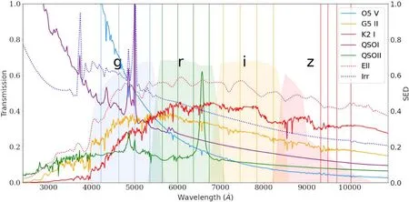
Figure 1.The transmission function of four filters from the CSST(shaded region),and the spectra energy distribution(SED)of objects that are used in our simulation.The crimson dotted line and blue dotted line represent the SED of an elliptical galaxy(Ell)and an irregular galaxy(Irr).The dodger blue,orange,and red solid lines represent three different types of star SEDs,which are O5 V,G5 II,and K2 I respectively.The purple and green solid lines indicate two different types of QSO SED(QSOI and QSOII).The vertical lines indicate the wavelengths where we have the simulated PSFs.

The PSFs are simulated on a 30×30 grid uniformly on the whole Field Of View (FOV).Each stamp of PSF simulation comprised of 512×512 pixels with pixel scaleAt each grid,there are simulated PSF images at four different wavelengths in each band.We do not find a strong variation of the size of the PSF over the FOV,while the ellipticity of the PSF varies rapidly (right panel of Figure 2).There are variations of the PSF at different wavelengths.The mean value of PSF ellipticity and size for the longest and shortest wavelength in our simulations is 4.71×10-3,6.43×10-3and 24.03,26.24 pixels respectively.Here we use the modulus of ellipticity.The wavelengths are indicated by the vertical lines in Figure 1.We show an example of the simulated PSF in the left panels of Figure 2.

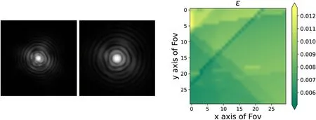
Figure 2.Left panel:two examples of simulated PSF of CSST at 4630 Å in the g band(left)and 7500 Å in the i band(right).The intensity is given in the log scale in arbitrary units.Right panel: the spatial distribution of the PSF ellipticity on the FOV at wavelength 7830 Å in the i band.

We chose two kinds of SEDs for the reference galaxies,three for the stars and two for the QSOs.The galaxy SED templates from Coleman et al.(1980): an elliptical galaxy that has a relatively red color and an irregular galaxy that has a blue color.The two distinguishing spectra can give us an up limit of the color and color gradient bias.For short,we dub the two galaxies as Ell and Irr respectively throughout the paper.The SED templates of stars were taken from Pickles (1998): the stars of type O5 V,G5 II and K2 I.O5 V have a blue color,K2 I has a red color and G5 II is somewhere in between.In addition,QSOs have point-like image morphology and can be misclassified as stars for the PSF estimation.We studied the color bias from QSO SED as well.The SED templates of QSOs are adopted from the SWIRE library,Polletta et al.(2007): a Type-1 QSO (QSOI) and a Type 2 QSO (QSOII).The probability of mis-classification of QSO to the star is difficult to estimate and depends on the observations.For example,one can reach high precision with spectra.In von Marttens et al.(2022),the classification of galaxy-star-QSO using the J-PLUS DR3 has been carried out.One million stars and 0.2 million QSOs have been identified.The result shows that using 12 photometric bands,they can reach a precision of 0.94 for QSOs.Given the high number density of QSOs,and even higher at high redshift,it is necessary to include the contamination of the QSOs.All the SEDs that we used are shown by the curves in Figure 1,in which all the SEDs are rescaled arbitrarily for better visibility.

Because we have only four simulated PSFs on different wavelengths in each band,further uncertainties exist in our estimates of the color bias.For example,as one can see from Figure 1,the strong emission line in the SED of QSOII around 6570 Å in therband cannot be covered.To account for most of the features in the SED,the linear interpolation on the pixel level between each pair of adjacent simulated PSFs is applied to the PSFs.These mocked PSFs are produced with the step of wavelength 10 Å.With the PSF at each wavelength and the SED templates,we generate the effective PSFs and calculate the color biasbc(Equation(6))between the star and the galaxy,and between the QSO and the galaxy.

In Figure 3,one example of the color biases between the Irrgalaxy and the three types of stars,or between the Irr-galaxy and the two types of QSOs are presented.We calculate the color bias on each grid over the whole FOV(30×30 grid)and show the magnitude distribution ofbc.Both the color bias of size and ellipticity has positive and negative values.We only show their absolute value for better visibility.The bias distributions ofRand ∈show differences in all bands using star SED or QSO SED.The bias varies dramatically between bands as well,especiallybcofR.bcof ∈5To distinguish the ellipticity of the PSF or galaxy,we use ellipticity only for that of the PSF,and use shear γ for that of the galaxy.is relatively large,one of the reasons is that the intrinsic ellipticity of the PSF is small～10-3.The absolute difference is～10-5,which gives the order of relative bias for ellipticity roughly 10-2.It shows less difference between the four bands.Similar distributions are shown when we use stars or QSOs to estimate PSF.Three major properties can be summarized from Figure 3: (1) In general,bcofRis smaller and has a narrower distribution over the FOV than that ofbcof ∈.(2)The color bias in the band of a short wavelength usually is greater than that of a longer wavelength.One can see from Figure 1,that there is more diversity at a shorter wavelength in the spectra of all the sources.(3) The strong emission line in SED can have a significant impact onbc.For example,an emission line of QSOI around 5000 Å can be redshifted intoiband when the QSO is atz～0.5.Thus,from the panel of QSOI(0.5)one can see that the bias in theiband is drastically large than that in the other cases.A similar situation is that there is an emission line of QSOII at 6570 Å.It will be redshifted into thezband when the QSO is atz=0.5.In additional tests,we check the difference of the SED between the star/QSO and the galaxy.A similar trend can be found as well.

Figure 3.The histogram of the color bias in the CSST g,r,i,z band using blue,green,orange and red colors respectively.The results between Irr and three types of stars(O5 V,G5 II,K2 I),as well as two types of QSOs(QSOI and QSOII),are shown.We use typical redshifts for QSOI and QSOII,which is 0.5(left)and 1.0(right).In each panel,from left to right is the color bias of R and ∈respectively.

3.2.Color Bias with Color and Redshift

Since the color bias simultaneously correlates with the SED of the galaxy and that of the star,and the color of the source can broadly reflect the trend of the SED,and the color of the galaxy and the star can provide a rough estimate of the bias.Such a relation has been studied using real data in the Subaru Strategic Program survey (Carlsten et al.2018).To study the relation to the CSST,we generate a synthetic galaxy SED library.Each synthetic galaxy SED in our mock library is generated by combining an Ell SED and an Irr SED.They are used to mimic the spectrum of the bulge and disk of the galaxy.Different weightings are employed for the two components,i.e.,SEDgal=wSEDEll+(1-w) SEDIrr,wherewstands for the weighting.Eleven steps ofwfrom 0 to 1 are selected in our mock library,and 21 redshift steps between 0 and 2 are used.The colorr-iis calculated from the integrated flux of the two neighboring bands.Since we do not employ any particular magnitude system,the zero-point of the color index is arbitrary.The resultingbcare averaged over the FOV for each weightingwand redshift combination and are shown in Figure 4.Three types of stars and two types of QSOs at different redshifts(z=0.5,1.0)are used for the SED of PSF.The color bias in theiband is shown.A clear uptrend ofbcofRcan be seen,i.e.,the redder the galaxy,the greater the size bias.Especially for the case of a red galaxy and a blue star,the bias ofRcan be up to～0.006.Thebcof ∈do not have an obvious trend.

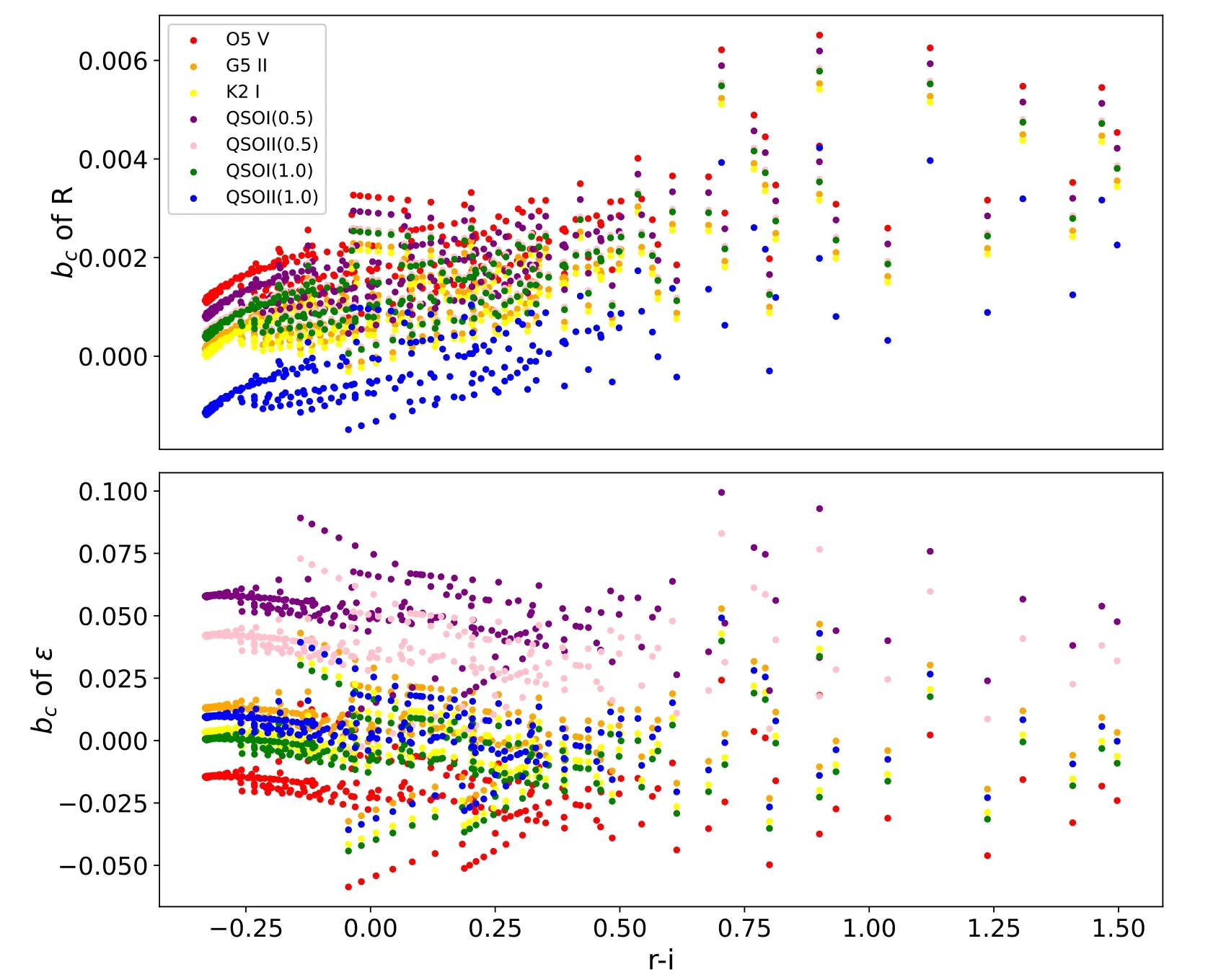
Figure 4.Color bias of the PSF between synthetic galaxies and stars/QSOs in the i band as a function of the color of galaxies.The red,orange and yellow points represent the bias using the star of type O5 V,G5 II and K2 I;the purple,pink,green,and blue points represent the bias using Type-I QSO(z=0.5),Type-II QSO(z=0.5),Type-I QSO(z=1.0),and Type-II QSO(z=1.0)respectively.Eleven synthetic galaxy SEDs between redshift[0,2]with step 0.1 are used.The zero-point of the color is arbitrarily set.

Moreover,the SED of the galaxies are redshifted when they are at a cosmological distance.The color bias,therefore,changes correspondingly,especially when the SED of the galaxy has strong emission lines.The bias in PSF can propagate into the weak lensing shear measurement (Paulin-Henriksson et al.2008;Cypriano et al.2010;Massey et al.2012),which is eventually important to us.We adopt the approach in Massey et al.(2012) to estimate the multiplicative biasmdue to the imperfect knowledge of the PSF,

whereRgalis the size of galaxy,RPSFis the size of the PSF,represents the bias offrom its true value andis the variance ofFor simplicity,we keepRPSF/Rgalas 1/1.5.The same as in the previous section,we calculate the average over the whole FOV for each redshift.Three types of stars and two types of QSOs atz=0.5 are used as references.We present the shear measurement error due to the color bias in Figure 5.The bias using the O5 V star is greater than the other cases in general.It agrees with our expectation since we find a strong difference in SEDs between O5 V and galaxies.Two main features can be seen here: (1)The order of magnitude of the shear bias is similar between the two types of galaxies.(2)The amplitude of shear bias decreases with the band,i.e.,We can see that the multiplicative systematic bias in shear measurement caused by color bias is smaller than typically current constraintm～10-2(Jarvis et al.2016;Mandelbaum et al.2018;Li et al.2023).However,Equation (8) only includes the contribution of second-order moments.As pointed out by Zhang &Mandelbaum (2022),Zhang et al.(2023),the higher order moments of the PSF can be a significant source of the shear bias in the upcoming surveys.The exact magnitude of such an effect requires sophisticated simulations,which will be left in future work.

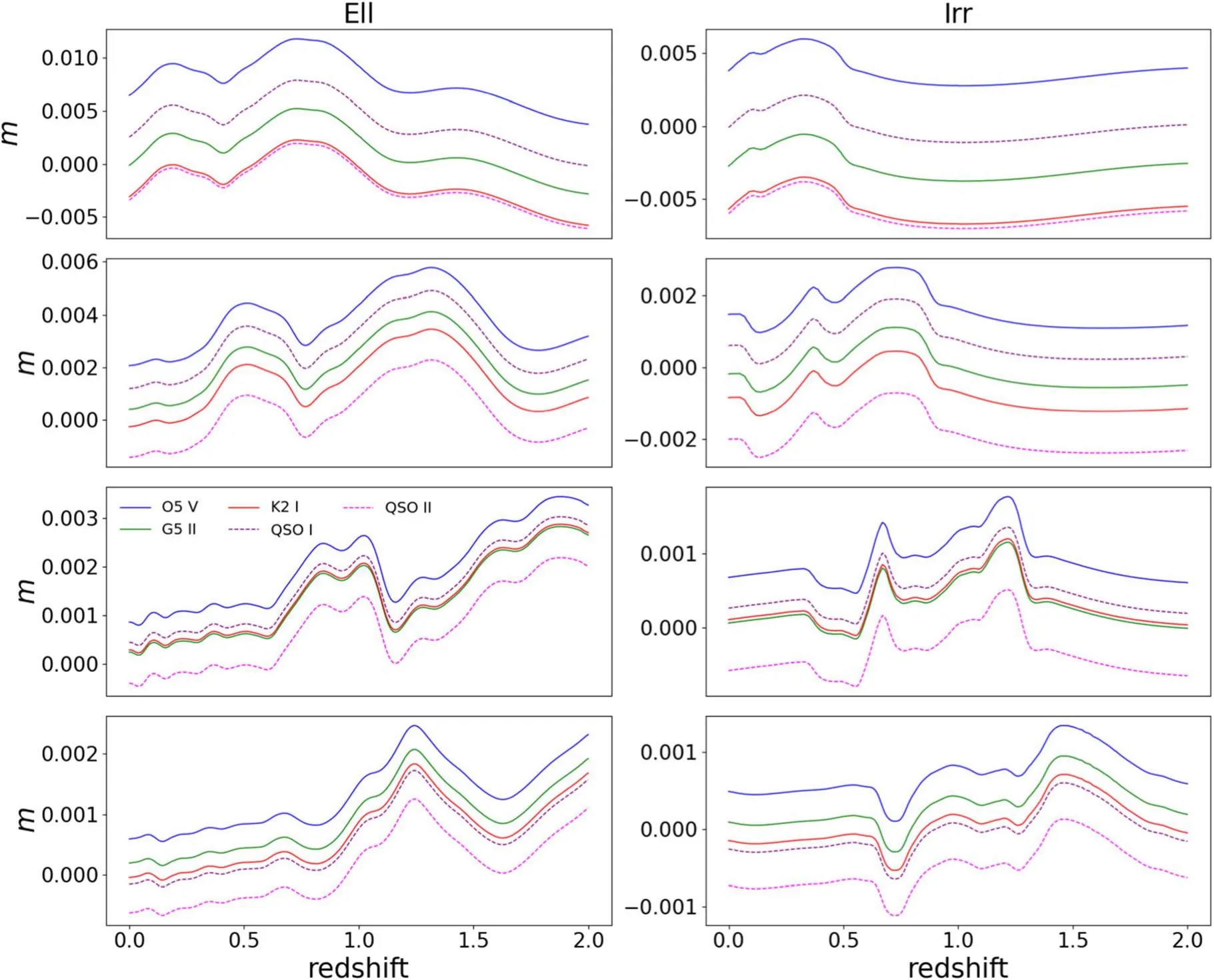
Figure 5.The multiplicative systematic bias of shear measurement due to the color bias vs.redshift.From top to bottom is the result in the g,r,i,z band respectively.In the left (right) column,the SED of an Ell (Irr) galaxy is used.Different SEDs of stars/OSQs are presented by different color curves.

The stars we used to estimate the PSF are local,i.e.,z=0,while the QSOs have a wide distribution of redshift.To see the color bias with different combinations of QSO redshift and galaxy redshift,we perform an additional test with the redshift range from 0 to 2 with a step of 0.01 for both galaxies and QSOs.Figure 6 shows the color bias between Irr and QSOII.From Figure 6,one can see thatbcofRis rough 10-3andbcof∈is about 0.03 in the most redshift combinations (relatively dark region).The color bias does not change drastically in different redshift combinations of the galaxy and the QSO in general.However,there are some vertical and horizontal bright stripes that appear on both left and right panels,which shows acute changes of the color bias at these redshift combinations,especially when the QSO atz～0.27(left panel,bias ofR)andz～0.05 or 0.14 (right panel,bias of ∈).It is due to the strong emission line of QSOII (at around 6570 Å) iniband at these redshifts.It can give a large weighting of the PSF at this wavelength.The wavelength dependence of the PSF size or PSF ellipticity is different,thus the stripe appears at different redshifts on the left or right panel.

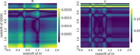
Figure 6.The heat map of the color bias between Irr and QSOII in the i band.The horizontal(vertical)axis is the redshift of the galaxy(QSO).From left to right are the bias of size and the bias of ellipticity.The redshift of the galaxy or QSO is in range from 0 to 2 with step 0.01.

We further compare the color bias between using the star or QSO as reference.The same redshift range is adopted for the QSO and galaxy.The result is shown in Figure 7.

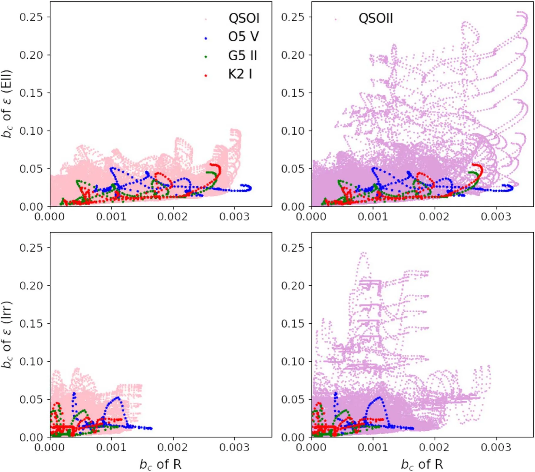
Figure 7.The distribution of color bias in the i band.Each point represents the color bias of R (horizontal axis) and bias of ∈(vertical axis) for one case of combination,the star with the galaxy or the QSO with the galaxy.Different redshifts for the galaxy and QSO are used.In the left(right)panels,we compare that of the stars with QSOI(QSOII).In the top(bottom)panels,the color bias is calculated with respect to the Ell(Irr)galaxy.Three different colors represent the bias using three SED of stars.

We find that the bias of ellipticity between the galaxy and QSO is bigger than that between the galaxy and star,especially for QSOII.The color bias of the size with stars is similar to that with the QSO.For both two kinds of galaxies (Ell or Irr),the color bias using QSOII is larger than using QSOI.The main reason for that is the strong emission line and the shape of the spectrum of QSOII.The difference between biases using the QSO or star can be explained by the same reason.

3.3.Calibration of Color Bias

The color bias can be calibrated from the SED or the color of the galaxy and star (e.g.,Eriksen &Hoekstra 2018).In this part,we present the calibration of the color bias.In order to isolate the color bias,the other noises,such as sky background or readout noise are not included here.There are possible couplings between the color bias and the other noises.But the color bias has systematic dependence on the SED of the star and galaxy.We use linearly interpolation from the two neighboring bands of the galaxy photometry to reconstruct the SED of galaxy Semboloni et al.(2013).The morphology of the galaxy is not included.We follow the same procedure that is used in Section 3.1 and obtain the reconstructed PSF (PSFrefor short) from the interpolated SED,then compare it with PSFgal.Forrbands,one can interpolate the SED either fromg,rbands or fromr,ibands.We reconstruct the SED both ways to calculate the color bias,and show the average color bias from two reconstructions.The same procedure is applied for theiband.In Figure 8,the color bias using reconstructed SED(black solid lines) is compared with the other cases.As one expects,there is a significant improvement,i.e.,the biases using the reconstructed SED are smaller than the others in most cases.One weakness of this method is that it cannot recover the acute structure in the galaxy SED,such as emission lines in the Irr galaxy.Moreover,the PSF model of wavelength dependence is required in this method.

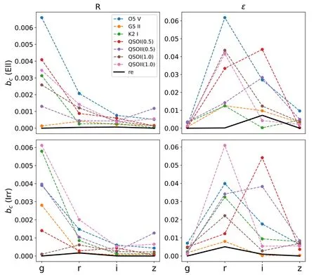
Figure 8.The mean color bias over the FOV in four bands of the CSST.From left to right is bc of R and bc of ∈.The Irr is used as the reference.The black solid lines present the bias using reconstructed SED of the galaxy.

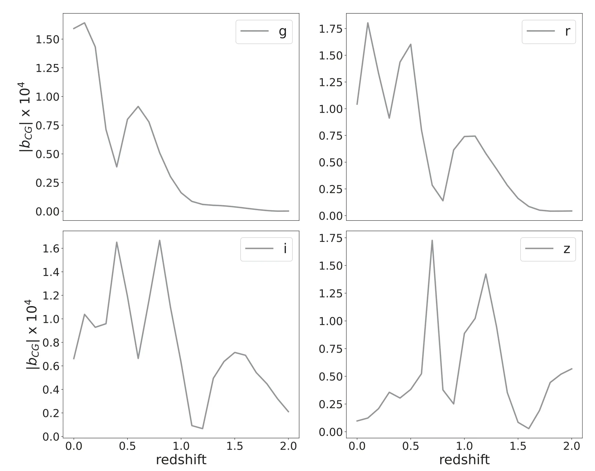
Figure 9.The color gradient bias as a function of redshift for the “big” galaxy in the g, r, i, z band of the CSST.

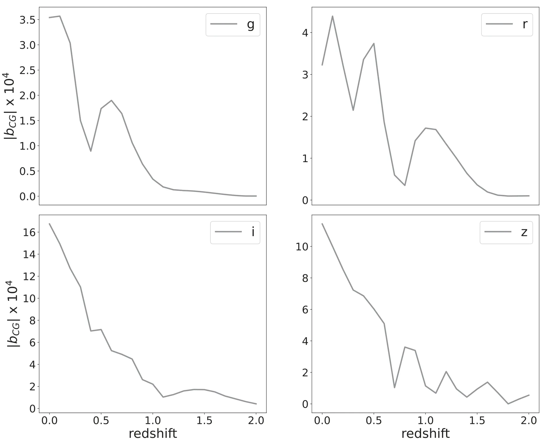
Figure 10.The same as Figure 9 but for the “small” galaxy.

4.Color Gradient Bias

The SED of a galaxy varies spatially,generating a color gradient.We estimate the shear measurement bias when the color gradient of the galaxy is ignored,i.e.,the CG bias.It has been shown that the CG bias depends on several factors,such as the measurement method,the relative size of the galaxy with respect to the size of the PSF,the pixel scale of the CCD,the transmission function of the filters etc.(e.g.,Voigt et al.2012;Semboloni et al.2013).On top of that is the color gradient of the galaxy.For example,if there is a great difference in the SED between the bulge and disk of the galaxy,one would expect a significant CG bias.More detailed discussions can be found in Semboloni et al.(2013).We evaluate the CG bias for CSST’s four filters following a similar approach in Er et al.(2018),and only introduce basic steps here(one can find more details from Figure 1 in Er et al.2018).Following the step in the Figure,one can generate the galaxy images without CG bias from the top flowchart: (1) convolve the image with PSF at each wavelength;(2) integrate the images over the band of wavelength;(3)deconvolve the image by the effective PSF;(4)shear the deconvolved image.In the bottom flowchart,one follows the real image process and can simulate the image with CG.The only difference is that the shear step is at the beginning.In reality,there is convolution with the effective PSF in the end for both top and bottom flow.Since we do not employ any particular PSF correction method,a direct deconvolution is used,and we cancel out the last convolution.Then we use the second-order brightness moment and Gaussian weighting function to measure the shear from these two kinds of images.

We combine a bulge and a disk to mimic the spatial variation of synthetic galaxy SED.Again we use an Ell galaxy SED for the bulge and an Irr galaxy SED for the disk.The image profiles are described by the Sérsic profile at each wavelength

whereI0is the central intensity,κ=1.9992n-0.3271,nis the Sérsic index,andqis the axis ratio,rhis the half-light radius.We taken=1.5 for the bulge andn=1 for the disk.The source galaxies are assumed to be circular initially.Two sizes of galaxies are considered in the first test.The size for the big galaxy and the small galaxy is given by the half-light radius of its bulge and disk:respectively.The total flux of the synthetic galaxy is normalized at the wavelength of 550 nm where the bulge and disk contain 25% and 75% of the flux respectively.A shear value (γ1=γ2=0.05) is uniformly used in all the tests.The PYTHON-based GalSim package (Rowe et al.2015) is used to simulate the galaxy image,which has been widely adopted in weak lensing studies (e.g.,Hoekstra et al.2016).The stamp size of each galaxy image is 512×512 pixels with the pixel size ofThe wavelength sampling interval is 1 nm.The PSF model is simply simulated by the Airy function,which shows a similar shape to the PSF in the CSSTiband(Shen et al.2022).The profile of the Airy disk is expressed as

whereI0is the maximum intensity at the center,κ is the aperture obscuration ratio,andJ1(x) is the first kind of Bessel function of order one;xis defined asWe take the CSST aperture diameterD=2 m and obscuration κ=0.1 in our simulation.In this study,we do not consider the evolution of the galaxies over the redshift,i.e.,we use the same angular half-light radius of the bulge and the disk for galaxies at different redshifts.But the size of synthetic galaxies vary due to the SEDs,i.e.,the ratio of the bulge-to-disk can change with the redshift.The spatial variation of CG bias over the FOV has not been taken into account.

We calculate the “shear” from the simulated images,and obtain the biasbCG.In Figures 9 and 10,we show thebCGversus redshift in each band with step Δz=0.1.Overall,the bias is small,especially in the big galaxy (＜1.8×10-4).It is slightly larger in the small galaxy (＜1.7×10-3).For both galaxies,the bias decreases with redshift,which agrees with the previous study,Er et al.(2018).The two peaks in the CG bias curves correspond to the two strong emission lines of Irr SED.We estimate the color gradient of our synthetic galaxy for comparison.In order to calculate the “color,” we split each band into two at the central wavelength of the bandwidth.The flux ratio between the two sub-bands of the galaxy image is taken as the color.The color difference between the central regionand the outer regionof the galaxy image is defined as the color gradient.We calculate the color gradient as a function of the redshift and find this relation shows a similar trend as that of CG bias.

In theiband andzband,there are unusually large biases in the case of a small galaxy at low redshift.The main reason is that the relative size of the galaxy with respect to that of the PSF becomes small and critical.From the relative strength of SED between the Ell and Irr galaxies (Figure 1),one can see that the synthetic galaxy is bulge-dominated and compacted at low redshift,and becomes disk-dominated and extended at high redshift.In additional tests with smaller PSF sizes,the CG bias shows similar behavior as that using large galaxies.

Moreover,we take different combinations between bulge size and disk size into account.Only the CSSTiband is performed in this part.Figure 11 shows the relation of CG bias with the size of two components of the synthetic galaxy.We use the bulge size fromand the disk size fromin each panel.Three redshifts(z=0.0,1.0,2.0)are used here.We can see that the CG bias is more sensitive to the bulge size than the disk size.There is rapid growth when the galaxy becomes small.

Figure 11.The relation between the color gradient bias and the galaxy size in the CSST i band.From left to right,three SEDs corresponding to different redshifts have been used.The different size combinations of the bulge and disk are used in each panel.The unit of the size is arcsec and is presented by the half-light radius.The size of the bugle decreases from 017 to 009,and the disk size decreases from 12 to 06.

5.Discussion and Summary

Weak gravitational lensing is one of the most powerful tools in modern cosmology.Next-generation weak lensing surveys,such as Euclid,CSST,LSST and WFIRST,will measure the weak lensing signal with unprecedented precision.The shape measurements benefit from the compact diffraction-limited PSF of the space-borne telescope.Thus small instrumental effects can become important and need to be carefully investigated.One of the effects is the wavelength dependence of the PSF.In this paper,we study two biases due to the chromatic PSF in the CSST weak lensing measurement.The first one is the color bias.The difference between the star SED and galaxy SED leads to the difference between the PSF obtained from star images and the PSF that smears the galaxy.The other one is the color gradient bias.It arises due to the spatial variations in the colors of galaxies.In our simulations,we find both of these two biases are small in most cases of the weak lensing measurement in the four optical filters of the CSST.

For the color bias,two types of SEDs are taken as references for the galaxy.One is an irregular galaxy,and the other one is an elliptical galaxy.Three types of SEDs of the star(O5 V,G5 II,K2 I)and two types of SEDs of the QSO(type I and type II)are used since the QSO has a point-like image and can be misclassified as the star.We study the color bias of the PSF size and ellipticity for the CSST.We find that the color bias of the size is one order of magnitude smaller than that of ellipticity in general.The order of magnitude distributions of the color bias of ellipticity show similarity in four bands,and covers a wide range.One of the reasons is that the ellipticity of the PSF is sensitive to the position on the field of view.Meanwhile the distribution of the color bias of size is centrally distributed in all bands and has widely separated among the filters.Two other properties can be found:(1)in the shorter wavelength filter,the color bias will be larger;(2) the strong emission line of the source galaxy has a big impact on the color bias.

We study the dependence of color bias on some other factors.By generating a synthetic galaxy SED library,we find that there is a positive correlation between the color bias of size and the color of the galaxy.Meanwhile the relation between the bias of ellipticity and galaxy color is not clear.In the color bias test for the galaxy at different redshifts,we do not find a large difference between the elliptical galaxy and the irregular galaxy.We also calculate the shear measurement error due to color bias,and find in all four bands,the shear measurement errors are small (＜1%).In the redshift combination of the galaxy and QSO,we find the color bias is significantly affected by the strong emission lines in the SED of galaxy and QSO.We perform calibration to the color bias by reconstructing the SED of the galaxy.We use the brightness of two neighboring bands and linearly interpolate the SED of the galaxy.The PSF based on the reconstructed SED provides a better estimate of the PSF,which is close to one that smears the galaxy.

For the color gradient bias,only the multiplicative bias is studied.We adopt the Airy profile to simulate the PSF and estimate the CG bias at different redshifts for four CSST bands.For galaxies at different redshifts,we not only consider the changing of the SED,but also the evolution of the galaxies.The CG bias is also small～10-4and decreases with redshift in general.Similar to that in the color bias,a strong emission line of the source galaxy can increase the CG bias.When the size of the galaxy becomes small,the CG bias also increases rapidly.Particularly in the CSSTiband andzband,the bias can be up to 1.7×10-3and 1.2×10-3respectively.The main reason is that the ratio between the PSF size and galaxy size is relatively large in these bands.Our results show that the CG bias in the CSST shear measurement is a subdominant effect for relatively big galaxies,but for small galaxies,in the CSSTiandzband CG bias can cause non-negligible systematic bias in the Stage-IV weak lensing survey.

In this study,we show that the chromatic effect in the PSF can be small in most cases of shear measurements.However,there are some exceptions one has to be careful of.For example,the misclassification of the QSO as the star and measuring shear from small-size galaxies.Moreover,there are some simplifications in our study.First,in our simulation,we only consider the optics of the CSST.Other instrumental effects,such as those from the detector,need to be included as well.The linear reconstruction method to calibrate the color bias needs to be processed for every galaxy,which will require massive computation cost.The relation between the color and the color bias can provide a neat estimate of the bias.The evaluation of the color gradient bias in this paper is based on the Airy profile.An estimate with realistic noise and calibration to other wider band filters(Liu et al.2023)will be important to the weak lensing measurement as well.

Acknowledgments

We would like to thank the referee for the comments and suggestions on our draft.This work was funded by the National Natural Science Foundation of China (NSFC) under Nos.11873006,11933002,11903082,and U1931210.We acknowledge the science research grants from the China Manned Space Project with Nos.CMS-CSST-2021-A01,CMS-CSST-2021-A12,and CMS-CSST-2021-A07.

ORCID iDs