Analytical Study of the Co-orbital Motion in the Circular Restricted Threebody Problem

Xinhe Shen, Tao Liu, and Xinhao Liao

1 Shanghai Astronomical Observatory, Chinese Academy of Sciences, Shanghai 200030, China; liutao@shao.ac.cn

2 Key Laboratory of Planetary Sciences, Chinese Academy of Sciences, Shanghai 200030, China

3 University of Chinese Academy of Sciences, Beijing 100049, China

4 School of Physical Science and Technology, ShanghaiTech University, Shanghai 201210, China

Abstract In the restricted three-body problem (RTBP), if a small body and a planet stably orbit around a central star with almost exactly the same semimajor axis,and thus almost the same mean motion,this phenomenon is called the coorbital motion,or equivalently,the 1:1 mean motion resonance.The classical expansion of the disturbing function is divergent when the semimajor axis ratio of the small body to the planet is close to unity.Thus, most of the previous studies on the co-orbital dynamics were carried out through numerical integrations or semi-analytical approaches.In this work,we construct an analytical averaged model for the co-orbital motion in the framework of the circular RTBP.This model is valid in the entire coorbital region except in the vicinity of the collision singularity.The results of the analytical averaged model are in good agreement with the numerical averaged model even for moderate eccentricities and inclinations.The analytical model can reproduce the tadpole, horseshoe and quasi-satellite orbits common in the planar problem.Furthermore, the asymmetry of 1:1 resonance and the compound orbits (Icarus 137:293–314) in the general spatial problem can also be obtained from the analytical model.

Key words: celestial mechanics – methods: analytical – minor planets – asteroids: general

1.Introduction

The co-orbital motion or 1:1 mean motion resonance is one of the most interesting topics of the three-body problem and has been extensively studied for more than 100 yr.The history of the co-orbital motion began with the work of Euler and Lagrange in the 18th century.In 1767, Euler found that the general three-body problem has three special solutions in which the three masses are collinear at each instant.In 1772,Lagrange found a second kind of special solutions to the general threebody problem in which the three masses form an equilateral triangle at each instant.In the circular restricted case, these special solutions correspond to the well-known Lagrangian equilibrium points:the collinear points L1,L2,L3;the triangular points L4and L5.The Lagrangian points L4and L5are linearly stable to small displacements when ∈＜0.0385, where∈=m2/(m1+m2) is the mass ratio of the system(Gascheau 1843).This implies that a small body can remain near L4or L5and thus stably share the same orbit with a planet.Such a small body is called a Trojan.The first Trojan asteroid,588 Achilles, which is librating around Jupiter’s L4, was discovered by Max Wolf of the Heidelberg Observatory in 1906.

The 1:1 mean motion resonance manifests itself in a variety of modes of motion.The different modes of motion can be distinguished according to the librational behavior of the resonant angle,l～λ λ= - ′, where λ andλ′ are the mean longitudes of the small body and the planet respectively.There are three elementary modes of co-orbital motion:(i)tadpole(T)or Trojan orbits,wherel～librates around L4or L5;(ii)horseshoe(HS)orbits,wherel～librates around L3with an amplitude larger than 180° encompassing L4and L5; (iii) quasi-satellite (QS)orbits,associated with a libration ofl～ around 0°.It is important to point out that the Lagrangian points L4and L5(i.e., the libration centers of the tadpole motion) are exactly located atl～ = ± 60° only when the small body’s orbit is circular and planar; for eccentric and inclined orbits of the small body the effective Lagrangianpoints L4and L5willbe displaced appreciablyfroml～ =± 60°(Namouni&Murray2000).Apart from these three elementary co-orbital orbit families, in the spatial case the quasi-satellite orbits can merge with horseshoe or tadpole orbits to form the stable compound orbits,H–QS,T–QS and T–QS-T (Namouni 1999; Namouni et al.1999;Christou 2000).The compound T–QS orbits, which are also called the large-amplitude tadpole orbits,librate around 0°with amplitudes less than 180° and encompassing L4or L5.In the compound T–QS-T mode,l～ librates around 0° with an amplitude larger than 180° encompassing L4and L5.A compound H–QS orbit corresponds to an asymmetric horseshoe-like libration around L3with a narrow opening ahead or behind the quasi-satellite domain.

A classical example of the tadpole motion is the Jovian Trojan population containing several thousand members.Trojan asteroids have also been found for Venus, Earth,Uranus and Neptune (see Greenstreet et al.2020, and references therein).The horseshoe motion was first observed in the Saturnian satellite pair Janus-Epimetheus during Voyager 1 flyby of Saturn in 1980 (Synnott et al.1981).There are several confirmed horseshoe objects coorbiting with the Earth (Kaplan & Cengiz 2020).The first known object following a quasi-satellite path was asteroid 2002 VE68which is a companion to Venus (Mikkola et al.2004).The Earth and Jupiter host the largest known number of quasi-satellites with at least eight in the solar system; while Venus, Saturn, Neptune and dwarf planet Ceres have one each (de la Fuente Marcos&de la Fuente Marcos 2016).Asteroid 3753 Cruithne, a coorbital of the Earth,is recognized to be moving in a compound H–QS orbit (Wiegert et al.1998; Namouni 1999).Another example of a H–QS orbit is Venus’co-orbital 2001 CK32(Brasser et al.2004).A probable candidate for the compound T–QS-T orbit is asteroid 2013 LX28, locked in 1:1 resonance with the Earth (de la Fuente Marcos & de la Fuente Marcos 2014).

Dermott & Murray (1981a, 1981b) studied the fundamental properties of quasi-circular tadpole and horseshoe orbits by means of the Jacobi integral and numerical integration; for the first time they gave a detailed description of the horseshoe motion of Janus-Epimetheus system with comparable masses.Yoder et al.(1983) derived an analytic approximation to the tadpole and horseshoe motions, which includes the secondorder correction to the 1:1 resonance caused by eccentricities and inclinations.A Hamiltonian secular theory for Trojan-type motion was constructed in the framework of the elliptic restricted three-body problem(RTBP)by Morais(1999,2001).Although these analytical theories presented in Yoder et al.(1983) and Morais (1999, 2001) are enough to describe the tadpole and horseshoe motions, they break down whenl～ =0 °and thus are not applicable to the quasi-satellite motion.Namouni (1999) investigated the co-orbital dynamics analytically using the Hill’s three-body problem and showed that in the spatial case recurrent transitions between horseshoe,tadpole and quasi-satellite orbits are possible.However, the Hill’s three-body problem is accurate only for sufficiently small mass ratios and small eccentricities and inclinations.Moreover,the asymmetry of the spatial 1:1 resonance with respect tol～ =0 °, resulting in the stable and asymmetric merger of horseshoe or tadpole with quasi-satellite orbits,is absent in the Hill’s problem.Thus,he reverted to the numerical integrations of the full equations of motion and then found new types of coorbital orbits referred as“compound orbits”(see also Namouni et al.1999).Later,following Schubarts numerical averaging of the Hamiltonian over the fast variable, Nesvorný et al.(2002)studied the global structure of the phase space of 1:1 resonance,and they replicated these new compound orbits in their semianalytical model.Such numerical averaging methods have been used in many researches on the co-orbital motion(e.g.,Beaugé& Roig 2001; Giuppone et al.2010; Sidorenko et al.2014;Pousse & Robutel 2017; Qi & de Ruiter 2020).In particular,Robutel&Pousse(2013)as well as Giuppone&Leiva(2016)derived an analytical Hamiltonian formalism adapted to the study of the dynamics of two planets in 1:1 resonance.However, since in their works the planetary Hamiltonian is literally expanded in powers of eccentricity and inclination with respect to zero eccentricity and zero inclination (i.e., the circular and coplanar orbit), the expansion of the planetary Hamiltonian is inherently singular at α=1 andl～ =0 ° (where α is the semimajor axis ratio of the two planets).This will give rise to incorrect phase space structures of 1:1 resonance for large/moderate eccentricities and inclinations.

In this paper, we develop an analytical averaged model which is valid in the entire regular co-orbital region and is applicable to both the planar and spatial problems.Using the analytical model we can recover all known co-orbital orbit families, including the tadpole, horseshoe, quasi-satellite, and compound orbits.The analytical averaged model is in good agreement with the numerical averaged model even for moderate eccentricities (＜0.3) and inclinations (＜30°).The paper is organized as follows.In Section 2, we introduce the analytical averaged model for the co-orbital motion of the circular RTBP.In Section 3,we study the phase space structure of the co-orbital dynamics using the analytical model.A comparison of the analytical averaged model with the numerical averaged model is presented in Section 4.Finally,we summarize the paper in Section 5.

2.The Analytical Model

We consider the circular restricted three-body problem consisting of a small body of negligible mass, a central star of mass M★and a planet of massm′ orbiting the star in a circular orbit.We shall use the standard notations a,e,i,ω,Ω,M and f for the semimajor axis, eccentricity, inclination,argument of perihelion, longitude of ascending node, mean anomaly, and true anomaly of the small body.We further define λ=M+ω+Ω and θ=f+ω+Ω to be the mean longitude and true longitude of the small body, respectively.Similar primed quantities refer to the planet.

The Hamiltonian of the circular restricted three-body problem is

where μ=GM★and G is the gravitational constant.R is the disturbing function given by

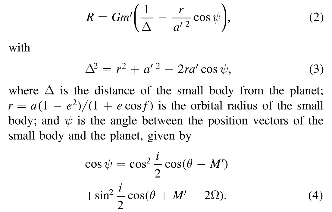
The first term of the disturbing function R is called the direct perturbation term which accounts for the gravitational interaction between the planet and the small body.The second term is called the indirect term which arises from the choice of the noninertial heliocentric frame.

It is convenient to describe the 1:1 mean motion resonance in the circular RTBP using the following canonical conjugate variables:

The Hamiltonian for the circular RTBP expressed in terms of canonical variables in Equation (5) reads

wheren′ is the mean motion of the planet.Note that the Hamiltonian in Equation (7) is independent ofh～, hence its conjugate momentumH～remain constant.

In the 1:1 resonance,the resonant anglel～ varies slowly with time compared to the mean motions of the small body and the planet.In fact,there are three dynamical timescales which have a hierarchical separation.The shortest timescale, associated with the orbital motions of the small body and the planet,is of order O(T)(where T is the orbital period of the small body).The intermediate timescale associated with the libration ofl～ is of order O (T ∈).The longest timescale associated with the secular evolution of ω and Ω is of order O(T ∈)(Wisdom 1985;Leleu et al.2018).This separation ensures that the short-period perturbations arising from the orbital motions do not affect the evolution of resonant and secular phases because their contributions tend to zero on average.Thus, the short-period terms containing M can be eliminated from the Hamiltonian in Equation (7) to simplify the problem, which is achieved by averaging the Hamiltonian over M.

The averaged Hamiltonian over the mean anomaly M is given by

The averaged Hamiltonian does not depend explicitly on time and therefore is autonomous.In order to find an analytical expression for the averaged Hamiltonian, first we expand the Hamiltonian in Equation (7) to second order in e and sin (i2).Then, averaging the expansion of the Hamiltonian (7) with respect to M, we obtain the analytical averaged Hamiltonian

A detailed derivation of the Hamiltonian (9) is presented in the Appendix.The averaged Hamiltonian can also be obtained by numerically integrating Equation (8).This numerical averaging treatment was first introduced by Schubart (1964)as a semi-analytical approach to the mean motion resonance.In this paper, we will call the numerical integration of the averaged Hamiltonian (8) “the numerical averaged model”and we call the Hamiltonian (9) “the analytical averaged model”.

3.Phase Space of 1:1 Mean Motion Resonance

In this section, we explore the phase space of the 1:1 mean motion resonance using the analytical averaged model.For the sake of simplicity, we will chose a system of units such that m=1,a′ =1 and G=1.Without loss of generality we setm′ = 10-3(a Jupiter-mass planet).

3.1.The Planar Case

In Figure 1, we show the phase portraits of the planar 1:1 resonance obtained in the analytical averaged model for e0=0,0.1, 0.2 and 0.3.For e0=0 (see Figure 1(a)), the phase space morphology is similar to the classical zero-velocity curves of the circular restricted three-body problem; the system has five equilibrium points, corresponding to the five Lagrangian points.L4andL5are exactly located atl～=60°and- 60°respectively,and L3atl～ =180°.In Figure 1(a)there are tadpole trajectories enclosing L4(or L5) and horseshoe trajectories enclosing L3, L4and L5.For e0=0.1, 0.2 and 0.3(see Figures 1(b)–(d)), there is an equilibrium point atl～ =0 °,and the quasi-satellite trajectories librating around the equilibrium point appear in the phase space.Moreover, as e0increases the size of the quasi-satellite domain increases,which is consistent with the previous works (see, e.g.,Nesvorný et al.2002; Pousse & Robutel 2017).It is clear in Figure 1 that the structure of the phase space for the planar case is symmetrical with respect tol～ =0 °.

When Δ=0 the Hamiltonian (1) as well as (8) becomes infinite, that is, the Hamiltonian (1)/(8) has a singularity that corresponds to the collision between the small body and the planet.However, the collision singularity has been removed from the analytical averaged Hamiltonian in Equation (9)(except for the case of e=0 and i=0°) due to the expanding manipulation of the analytical Hamiltonian.Hence there are no collision curves in Figures 1(b)–(d).This is a difference difference between the analytical averaged model and the numerical averaged model.In fact,the averaging method is not applicable to the dynamics in the neighborhood of the collision singularity (i.e., the Hill region of the planet) because the hierarchical separation between the timescales of the different variables breaks down in the Hill region (Robutel et al.2016;Pousse & Robutel 2017).Thus, the averaged model, whether analytical or numerical, cannot give real phase trajectories in the vicinity of the collision curves.This is an inherent drawback of the averaged method.

We can write a=1+Δa as the small body is coorbiting with the planet.Moreover, in our case:m′ ≪ Δa≪1.Thus,according to Equation (9) the phase trajectories can be approximately described by Wajer (2009)

Hence the shape of R*is crucial because the extrema of R*define the location of stable and unstable equilibrium points.The minima of R*define the stable equilibrium points, i.e.,libration centers around which there are the librating trajectories; while the maxima define the unstable equilibrium points (saddles) (Gallardo 2006).We define

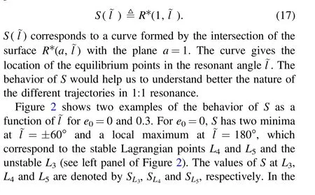
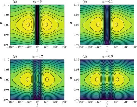
Figure 1.The phase portraits of the planar 1:1 resonance in the(a ,l～ )plane for e0=0,0.1,0.2 and 0.3.The curves represent the level curves of the Hamiltonian (9),and the background color maps represent the variation of the value of the Hamiltonian (9).

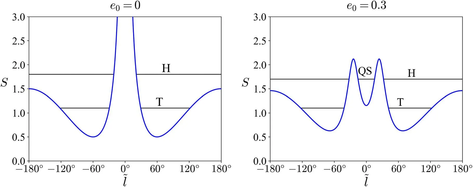
Figure 2.S ( l～) as a function of l～ for e0=0(left)and 0.3(right)in the planar case.T,H and QS denote tadpole,horseshoe and quasi-satellite orbits,respectively.The black horizontal lines correspond to the constant values of C.

Figure 3.The phase portraits of the spatial 1:1 resonance in the (a ,l～ )plane for a selection of values of e0, i0 and ω0.The curves are the level curves of the Hamiltonian (9),and the background color maps represent the variation of the value of the Hamiltonian (9).The red lines in(b)–(d)denote the compound H–QS,T–QS-T and T–QS orbits, respectively.

3.2.The Spatial Case

Figure 3 shows the phase portraits of the spatial 1:1 resonance obtained in the analytical averaged model for a selection of reference elements.In Figure 3(a) the quasisatellite domain disappear and there are only tadpole and horseshoe orbits.In this case the minimal angular separations of the horseshoe orbits could reach very small value (～0°).However,these horseshoe orbits might be unstable because the equilibrium point atl～ =0 is a saddle(Figure 4(a)),near which chaos occur.In Figure 3(b),the compound H–QS orbits appear as a result of the merger of horseshoe orbits with quasi satellite orbits.The H–QS orbit has a horseshoe-like trajectory but enclosing the quasi-satellite domain and has a narrow opening to the left ofl～ =0 ° (see the red line in Figure 3(b)).In Figures 3(c) and (d), there are compound T–QS-T orbits formed by the merger of the quasi-satellite orbits with the L4and L5tadpole orbits.The T–QS-T orbit makes the transfer of the small body from L4tadpole region to L5tadpole region possible,and vice versa.In Figure 3(d),we show an example of the compound T–QS orbit which is formed by the merger of the quasi-satellite and tadpole orbits.From the Hamiltonian in Equation (9) we note that, in the spatial case, only when cos 2ω=0 and ±1 the following relationship holds

Figure 4.S ( l～) as a function of l～ for a selection of reference elements same as in Figure 3.

This implies that in the spatial case the structure of the phase space is generally asymmetrical with respect tol～ =0 ° (for instance, Figures 3(b) and (d)).

In the spatial case, the collision event occurs only when the orbits of the small body and the planet interact at the ascending or descending node of the small body’s orbit.This requires that ω must satisfy (Nesvorný et al.2002)

Thus, there is generally no collision singularity except for specific values of ω.The collision singularity is replaced by the local maxima of the Hamiltonian as well asS(l～).The existence of the local maxima and the asymmetry of the Hamiltonian lead to the appearance of the compound orbits(Figure 4).

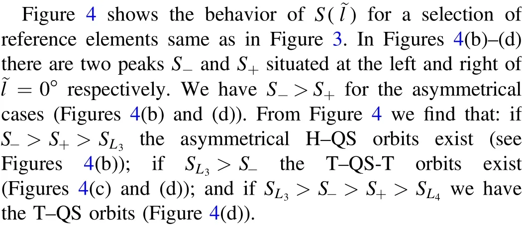
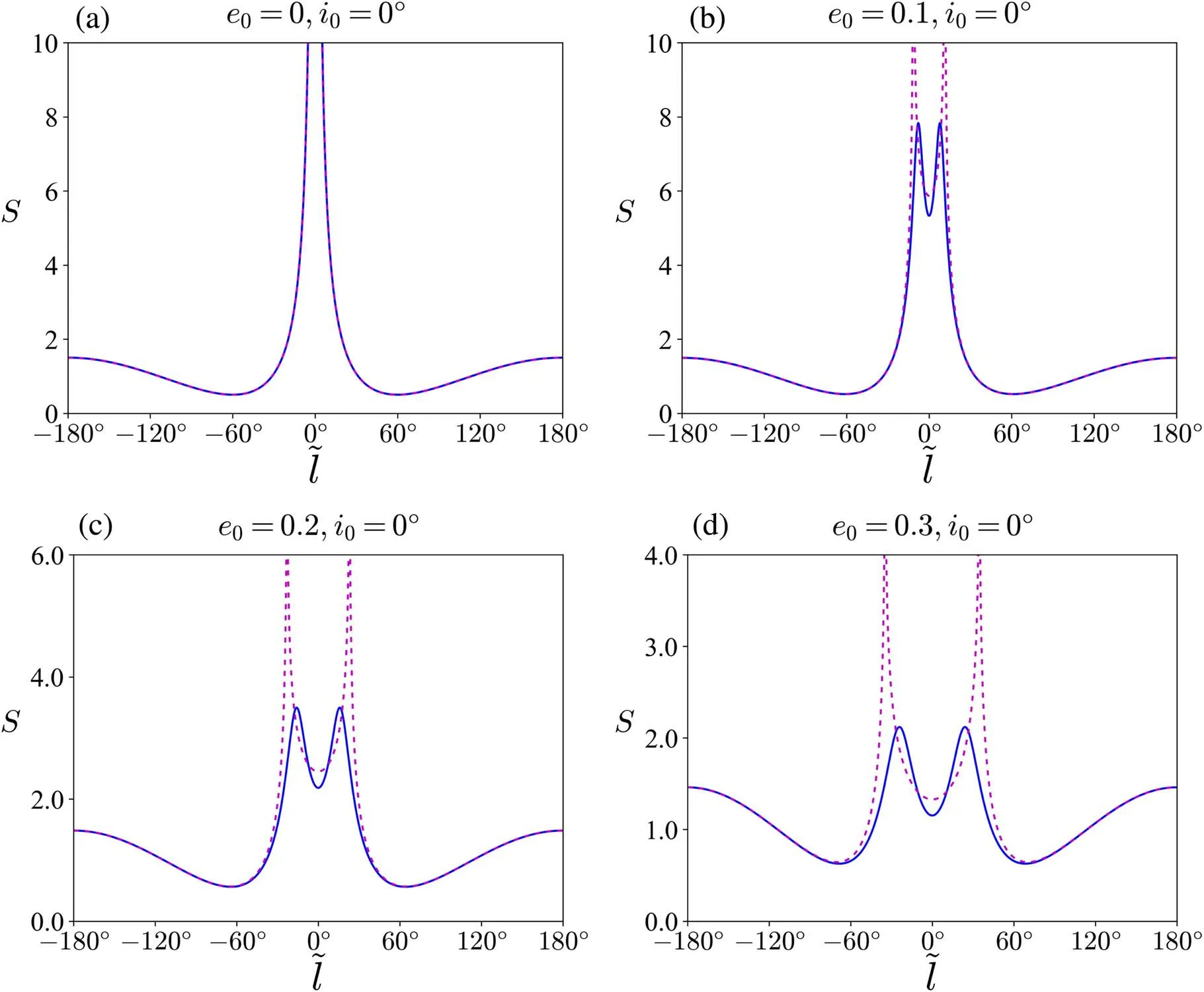
Figure 5.A comparison of the behavior of S between the analytical averaged model(solid lines)and the numerical averaged model(dashed lines)for the planar case.

4.Comparison with the Numerical Averaged Model

In this section we compare the analytical averaged model with the numerical averaged model.Note that the only difference of the two models is in the averaged disturbing functionR.Therefore,by comparing the behavior of S between the two models we can evaluate how the analytical averaged model agrees with the numerical averaged model.

A comparison of the behavior of S in the analytical and numerical averaged models for the planar case is shown in Figure 5.We see that the analytical averaged model is in complete agreement with the numerical averaged model for e0=0 (Figure 5(a)).Both models give a collision singularity atl～ =0 °.

Figure 7.The same as Figure 5 but for the spatial case.

For e0＞0, the collision singularity has been removed from the analytical averaged model and is replaced by the local maxima, while the numerical averaged model has two singularities at both sides ofl～ =0 ° (see Figures 5(b)–(d)).However, as illustrated in Section 3.1, both the analytical and numerical averaged models are not valid in the vicinity of the collision singularity, and neither of them can reflect properly the real dynamics in that region.Thus, this inconsistency between the two models may be ignored.Except near the collision singularity,the analytical averaged model agrees with the numerical averaged model well even for e0=0.3(Figures 5(b)–(d)).

The minima of S define the location of the Lagrangian points L4and L5.Thus,by finding the root of the equationdS dl～ =0 ,we can determine the displacement of the location of the Lagrangian point L4(or L5) froml～ = 60° (orl～ = 300°) for different values of e0.The result is shown in Figure 6.We can see that the Lagrangian point L4drifts outward froml～ =60 °with increasing e0for both the numerical and analytical averaged models.Importantly, for e0＜0.3 there is a quite small deviation between the analytical model and the numerical averaged model.

Figure 7 provides a comparison of the analytical averaged model with the numerical averaged model for the spatial case for a selection of reference elements, the same as that in Figure 3.It is clear from Figure 7 that for the moderate eccentricities and inclinations the behavior of S of the analytical averaged model is basically consistent with that of the numerical averaged model, although there are quantitative differences especially in the peaks S-and S+and the local minimum S0.

In the numerical averaged model, the peak S-actually corresponds to the minimum relative distance,Δmin, between the small body and the planet.Δminis a function of a, e, i and ω.For a=1, e=0.3, from Equation (19) we get ω ≈72°.5 for which the collision singularity occurs.This means that as ω →72°.5 the minimum relative distanceΔmintends to zero.Figure 8 shows that for the case of e0=0.3, i0=30° there is considerable disagreement between the analytical and numerical models when ω0is close to the value of 72°.5.In Figure 8,the numerical averaged model gives a very high and sharp peak S-to the left ofl～ =0 °for ω0=60°and 72°,corresponding to quite small values of Δmin;and yet the analytical averaged model gives a low and soft peak S-.This is because in the analytical averaged model the local maximum S-has been softened as a result of the elimination of the collision singularity.The softening maximum S-cannot reach a very large value.

Figure 8.The behavior of S of the analytical averaged model (solid lines) and of the numerical averaged model (dashed lines) for small values ofΔmin.

From the behavior of S shown in Figure 8 we see that the analytical averaged model gives the compound T–QS-T orbits;however, due to the existence of the sharp peak S-, there are the compound H–QS orbits instead of the T–QS-T orbits in the numerical averaged model.Consequently, the phase-space structure of the numerical averaged model is now qualitatively different from that of the analytical averaged model.This indicates that in such cases the analytical averaged model is not sufficient to describe the co-orbital dynamics especially for the compound orbits.However, from Figures 5, 7 and 8 we note that the analytical averaged model is always a good approximation to the tadpole and horseshoe motions.

5.Conclusions

In this paper we focused on the co-orbital motion in the circular restricted three-body problem, which consisted of a massless small body moving around a central star and perturbed by a planet in a circular orbit.We developed an analytical model adapted to the planar and spatial 1:1 resonance and valid in the entire con-orbital region.It takes two main steps to construct the model: first, we expanded the Hamiltonian of the circular restricted three-body problem to the second order in the eccentricity and inclination of the small body; then we averaged the result with respect to the mean anomaly of the small body and we obtained an analytical averaged Hamiltonian.

For the planar 1:1 resonance, our analytical averaged model can recover three classical types of the co-orbital motion:tadpole, horseshoe and quasi-satellite orbits.Moreover, the analytical model shows that as the eccentricity increases the quasi-satellite domain becomes larger and larger, which is consistent with the previous works.The shift of the Lagrangian points L4and L5was also observed in the analytical model.For the spatial 1:1 resonance, the analytical model reveals that the phase space structure is generally asymmetrical.There are the compound H–QS, T–QS and T–QS-T orbits which are formed by the merger of the quasi-satellite orbits with the horseshoe or tadpole orbits.The appearance of these compound orbits is due to the existence of the local maxima and the asymmetry of the Hamiltonian.

Comparison with the numerical averaged model shows that our analytical averaged model is valid even for the moderate eccentricities (～0.3) and inclinations (～30°).However, the analytical averaged model becomes a poor approximation to the dynamics in the vicinity of the collision singularity,for two reasons.First, the averaged method is not applicable to the motion inside the Hill region in which the timescales of the different degrees of freedom of the system are not separated well.Second, in the the analytical averaged model the local maxima of the Hamiltonian are softened as a consequence of the fact that the collision singularity is removed from the Hamiltonian.The softening maxima cannot reach a very large value when the minimum relative distance approaches zero,which would lead to the co-orbital dynamics qualitatively different from that of the numerical averaged model.

This paper may be helpful for relevant researches.For example, we can exploit the analytical model to calculate the oscillation amplitude and period of the co-orbital orbits.The averaged analytical model can be further used to study the secular stability of the co-orbital motion (especially for the tadpole and horseshoe orbits).Specifically,we can analytically study the orbital stability of the Trojan asteroids in tadpole orbits around the L4and L5Jovian Lagrangian points.We want to examine whether the number asymmetry of the L4and L5Jovian Trojans is related to the stability of the co-orbital motion at the L4and L5points.Moreover, using the analytical model we may provide a qualitative analysis of the secular stability of some recent found asteroids co-orbiting with the Earth(Borisov et al.2023).According to the analytical Hamiltonian, we may develop a secular formalism of the circular RTBP to study the secular evolution of the eccentricity and inclination of the coorbital objects.Furthermore, the co-orbital motion in the elliptic restricted three-body problem may also be approached analytically by using the methods presented in the paper.

Acknowledgments

We thank the anonymous referee for helpful comments and suggestions for improving this paper.The work is supported by the National Natural Science Foundation of China (NSFC)(grant No.11973010).

Appendix

Analytical Expression for the Averaged Hamiltonian

The averaged Hamiltonian is given by Substituting Equations (A13) and (A14) into Equation (A4)and averaging over the mean anomaly M(and keeping terms up to order e2), we obtain

with

which provides a better approximation for the 1:1 resonance when the small body approaches the planet closely.From Equations Equation (A7) and Equation (A8) it is easy to find