Unprecedented Heatwave in Western North America during Late June of 2021: Roles of Atmospheric Circulation and Global Warming

Chunzai WANG, Jiayu ZHENG,5, Wei LIN, and Yuqing WANG

1Southern Marine Science and Engineering Guangdong Laboratory (Guangzhou), Guangzhou 511458, China

2State Key Laboratory of Tropical Oceanography, South China Sea Institute of Oceanology, Chinese Academy of Sciences,Guangzhou 510301, China

3Innovation Academy of South China Sea Ecology and Environmental Engineering, Chinese Academy of Sciences,Guangzhou 510301, China

4University of Chinese Academy of Sciences, Beijing 100049, China

5State Key Laboratory of Numerical Modeling for Atmospheric Sciences and Geophysical Fluid Dynamics,Institute of Atmospheric Physics, Chinese Academy of Sciences, Beijing 100029, China

ABSTRACT An extraordinary and unprecedented heatwave swept across western North America (i.e., the Pacific Northwest) in late June of 2021, resulting in hundreds of deaths, a massive die-off of sea creatures off the coast, and horrific wildfires.Here,we use observational data to find the atmospheric circulation variabilities of the North Pacific and Arctic-Pacific-Canada patterns that co-occurred with the development and mature phases of the heatwave, as well as the North America pattern,which coincided with the decaying and eastward movement of the heatwave.Climate models from the Coupled Model Intercomparison Project (Phase 6) are not designed to simulate a particular heatwave event like this one.Still, models show that greenhouse gases are the main reason for the long-term increase of average daily maximum temperature in western North America in the past and future.

Key words: heatwave, climate change, atmospheric circulation pattern, Pacific Northwest

1.Introduction

Western North America (i.e., the Pacific Northwest of the United States and Canada), known for its temperate weather in June, normally has average high temperatures in the comfortable 18°C to 24°C range.However, western North America experienced an extreme heatwave in late June and early July of 2021, resulting in record temperatures in many places.In particular, Lytton, British Columbia broke Canada’s all-time record on 30 June when the temperature topped 49.5°C.This heatwave is also responsible for hundreds of deaths, a massive die-off of sea creatures off the coast, and a spate of horrific wildfires (https://en.wikipedia.org/wiki/2021_Western_North_America_heat_wave; Overland, 2021).Investigating and understanding the causes of this heatwave are both scientifically and socially important.

Some studies indicate that increasing trends in the frequency, duration, and intensity of heatwaves have accelerated on global and regional scales under global warming(Perkins et al., 2012; Perkins-Kirkpatrick and Lewis, 2020;Wang et al., 2020).There is increasing evidence that anthro-pogenic forcing, such as the forcing of rising greenhouse gases, is having an impact on heatwaves (IPCC, 2013,2021; Wang et al., 2020; Seong et al., 2021).In addition to external forcing, internal variability may also affect the changing nature of heatwaves.Changes in temperature and heatwaves are obviously related to climate modes and atmospheric circulations (Lau and Nath, 2012; Li and Ruan,2018; Li et al., 2019).Zheng and Wang (2019) identified seven atmospheric circulation patterns and combined these patterns along with global warming to explain summer surface air temperature variations in the Northern Hemisphere.Horton et al.(2015) showed that although a substantial portion of the observed change in extreme temperature occurrence has resulted from thermodynamic changes, extreme temperature trends have also been altered by recent changes in atmospheric circulation patterns.Some studies have also shown that heatwaves can be modulated by sea surface temperature(SST) anomalies.SST anomalies can remotely influence summer heatwave variabilities over land by generating severe convection and triggering atmospheric teleconnections (Wu et al., 2012; Wang et al., 2017; Chen et al., 2019; Deng et al.,2019).

This paper uses data from observations and climate models to study physical processes that may be responsible for the Pacific Northwest heatwave that occurred in late June of 2021 from the perspectives of internal variability and external forcing.Section 2 introduces the datasets, climate models,and methodologies used in this paper.Section 3 shows the results analyzed from observational data and climate model outputs.Finally, section 4 provides a summary and discussion.

2.Data and methods

2.1.Observational data

The daily atmospheric dataset used in this study is from the National Center for Environmental Prediction/National Center for Atmospheric Research (NCEP/NCAR) reanalysis I, which includes surface air temperature at the sigma-995 level, geopotential heights, horizontal and vertical winds on a 2.5° × 2.5° grid (Kalnay et al., 1996).To capture atmospheric circulation patterns associated with the Pacific Northwest heatwave, the analyses were performed from 1979-2021 since the satellite data were introduced in the late 1970s (Sturaro, 2003).The National Oceanic and Atmospheric Administration (NOAA) Optimum Interpolation Sea Surface Temperature (OISST), which is v2.0 from 1982-2015 and v2.1 from 2016-21, is used to detect the relationship between atmospheric circulation and SST(Reynolds et al., 2007).

The Global Historical Climatology Network-Daily(GHCND) dataset is also used in this study (Menne et al.,2012).Daily maximum temperature (Tmax) data at the surface in a region (40°-60°N, 100°-130°W) of western North America from 15 June to 15 July during 1951-2021 are selected.The Tmaxanomalies are calculated by using the period of 1961-90 as the climatology.

2.2.Climate models

Model-simulated daily near-surface air maximum temperature (“tasmax”) from the Coupled Model Intercomparison Project Phase 6 (CMIP6) is also used in this study.Historical simulations are performed to represent the response to all external forcing (ALL) by using 17 historical simulations from 7 models (Table 1).The time period used in this study for the historical simulations is 1951-2014.In addition, 17 simulations from 7 models are used for projections under Shared Socioeconomic Pathways scenarios (SSP2-4.5) during 2015-2100 (Table 1).The Detection and Attribution Model Intercomparison Project (DAMIP) is a part of the CMIP6.DAMIP contains three tiers of simulations, which cover 14 types of experiments driven by various forcings,such as well-mixed greenhouse-gas-only (GHG) historical simulations, anthropogenic-aerosol-only (AER) historical simulations, and natural-only (NAT) historical simulations(Gillett et al., 2016).Here, we use 17 historical simulations from 7 models under GHG forcing, AER forcing, and NAT forcing during 1951-2020 from DAMIP (Table 1).Similarly, six simulations from two models (CanESM5 and MIROC6) under GHG forcing, AER forcing, and NAT forcing from SSP2-4.5 are used for future projections during 2021-2100.Models are excluded if they do not provide the results of relevant simulations under GHG, AER, and NATforcings.Following the spatial resolution of observations,all daily maximum temperature data are interpolated into a uniform grid (2.5° × 2.5°) before analysis.

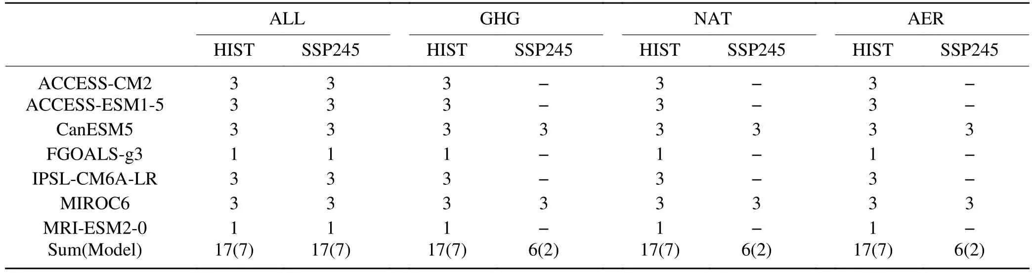
Table 1.List of CMIP6 climate models used in this study.Numbers represent the number of members for the ALL, GHG, AER, and NAT forcings.

The probability density functions (PDFs) of the Tmaxanomalies are calculated to estimate the probability of the observed 2021 heatwave.The PDFs are estimated by the kernel smoothing function (Ma et al., 2017).The probability ratio (PR) and the fraction of attributable risk (FAR) are used to quantitatively assess the contributions of anthropogenic influence to the observed 2021 heatwave and are defined as follows (Stott et al., 2004; Fischer and Knutti,2015; Ma et al., 2017): P R=PALL/PNAT;FAR=1-PNAT/PALL.PALLandPNATrepresent the probability of exceeding the extreme event like the observed 2021 heatwave under ALL and NAT simulations.The 95% confidence intervals of PR and FAR are estimated by the bootstrap sampling method (Ma et al., 2017).

2.3.Empirical orthogonal function analysis

Daily 300-hPa geopotential height variations during June-July for the period of 1979-2021 are adopted in this study to examine atmospheric circulation patterns associated with the heatwave in western North America.First, daily 300-hPa geopotential height anomalies are calculated relative to the climatological mean for 1979-2021.Second, geopotential height anomalies are weighted by latitude (cosine of latitude).Third, daily 300-hPa geopotential height anomalies during June-July for the period of 1979-2021, a span of 2623 days, are used to perform the empirical orthogonal function(EOF) analysis.The EOF modes identify the atmospheric circulation patterns, and their corresponding principal component (PC) time series are defined as the atmospheric circulation pattern indices.

2.4.Atmospheric wave activity flux

In this study, atmospheric wave flux is used to demonstrate atmospheric wave activity fluxes associated with atmospheric circulation patterns.First, daily 300-hPa stream function anomalies are calculated relative to the climatological mean for 1979-2021.Second, the stream function anomalies associated with atmospheric circulation patterns are obtained as the stream function anomalies regressed onto atmospheric circulation pattern indices.Third, the wave flux is computed based on the formula given in Takaya and Nakamura (Takaya and Nakamura, 2001):

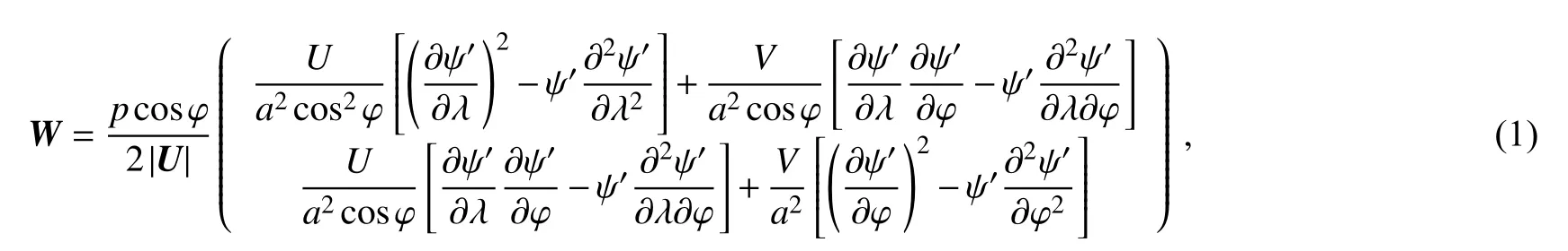
wherepis the normalized atmospheric pressure (pressure/1000 hPa), a is the earth’s radius, U and V are climatological mean zonal and meridional winds, |U| is the speed of the climatological mean winds, ψ′denotes the stream function anomalies, and (φ, λ) are latitude and longitude, respectively.

2.5.Extreme fitting method

A linear fitting method is usually used to reconstruct atmospheric variable anomalies (Wang et al., 2013).In this study, this method is used to reconstruct anomalies when the value of atmospheric circulation pattern indices is relatively large, which is termed the extreme fitting method.First, the slope patterns (SLs) are calculated as the fields of regression coefficients onto the atmospheric circulation pattern indices when the atmospheric circulation pattern indices are greater than 1.2σor less than -1.2σ(σis the standard deviation).The intercept patterns (INs), which are the fields of intercepts, are also obtained when the atmospheric circulation pattern indices are greater than 1.2σor less than-1.2σ.To emphasize extreme atmospheric circulations and their effects on the heatwave in western North America, the SLs and INs are set to zero when the atmospheric circulation pattern indices are between -1.2σand 1.2σ.Second, the daily 300-hPa geopotential height (GHT) and surface air temperature (SAT) anomalies are calculated as follows:

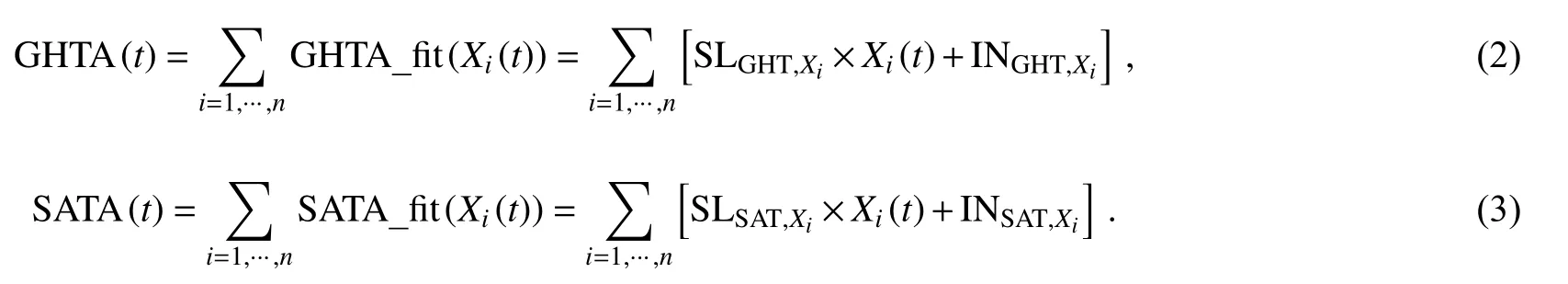
Here, Xidenotes the North Pacific, Arctic-Pacific-Canada,and North America pattern indices.For example,SLGHT,NPindex＞1.2σis calculated as the regressed daily 300-hPa geopotential height anomalies onto the North Pacific pattern index when the North Pacific pattern index is above 1.2σ.Thus, daily 300-hPa geopotential height and surface air temperature anomalies can be reconstructed using the atmospheric circulation pattern indices and their corresponding slope and intercept patterns.

3.Results

3.1.Development and decaying of the heatwave

The devastating heatwave was caused by a heat dome of high pressure (or anticyclone) over western North America.The heat dome gets its name because hot air is trapped by a high-pressure system; as the hot air is pushed back to the ground, it heats up even more (Ramamurthy et al., 2017).As shown in Fig.1, the extreme high-temperature anomalies over western North America were associated with positive 300-hPa geopotential height and negative 500-hPa vertical velocity anomalies (positive omega).These indicate that the anticyclone and downward motion gave rise to air warming by adiabatic heating during compression of sinking air(Black et al., 2004).In other words, the heat dome acted as a lid on the atmosphere, which trapped the hot air trying to escape and warmed it even more as it sank.The stronger the heat dome gets, the hotter the near-surface temperature is,and vice versa.

In addition to the anticyclone and sinking motion, the heatwave is also associated with the wind change in the tropopause.In a normal condition, a narrow band of very strong westerly air currents near the altitude of the tropopause, called the jetstream, is relatively flat in the middle latitudes.During the heatwave, the flat jetstream is distorted into a wavy pattern and even an omega shape at the peak of the heatwave (Fig.1d).

The heat dome first became evident on 24 June and gradually vanished after 2 July (Fig.1).The positive 300-hPa geopotential height anomalies near the coast of North America were aligned with the negative geopotential height anomalies in the North Pacific and the Arctic, suggesting that theheat dome was related to the atmospheric variations in the west of and north of North America.As shown later by atmospheric wave activity flux, the heat dome of western North America in late June of 2021 did originate from both the North Pacific and the Arctic.

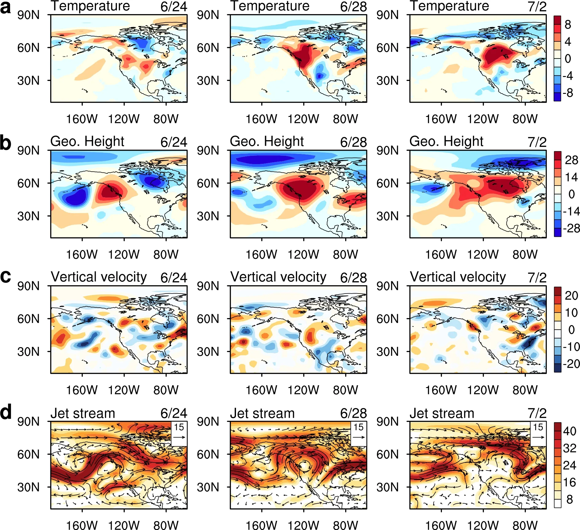
Fig.1.The Pacific Northwest heatwave from 24 June to 2 July 2021.(a) Daily surface air temperature anomalies at sigma-995 level (shading; units: °C).(b) Daily 300-hPa geopotential height anomalies (shading; units: 10 gpm).(c) Daily 500-hPa pressure vertical velocity anomalies (shading; positive values denote downward motion; units: 10-2 Pa s-1).(d) Daily 300-hPa wind speed (shading; units: m s-1) and horizontal wind field (vectors; units: m s-1).

To better understand the formation and development of the heat dome, we perform an empirical orthogonal function(EOF) analysis of the 300-hPa geopotential height by using the daily data from June-July over the period 1979-2021(Fig.2).Notably, these EOF modes are not overly sensitive to the choice of domain.Based on the horizontal structures and temporal variations of geopotential height and air temperature (Figs.2 and 3), we select the EOF1, EOF4, and EOF8 modes, which can be used to explain the heatwave in late June of 2021.As shown in Fig.3, the regressed surface air temperature anomalies onto PC1, PC4, and PC8 show positive values in western North America.In addition, it will be shown later that the reconstructed geopotential height and temperature anomalies, using the indices of these three patterns, well-resemble the observed distributions, indicating that the EOF1, EOF4, and EOF8 modes are related to the Pacific Northwest heatwave in late June of 2021.

The other five EOF modes are not chosen for the reasons as follows.First, the PC time series of the EOF2, EOF5, and EOF6 modes are weak from 24 June to 2 July 2021.Second,the spatial pattern of the other five modes does not resemble the observations.For example, the EOF3 mode is characterized by a meridional dipole with one low-pressure center over the Pacific and one high-pressure center over the Arctic, whereas the EOF7 mode consists of five pressure centers over the study region.These spatial patterns of geopotential height anomalies do not share similar structures to the observations.Third, the PC time series of the other five modes do not keep pace with the evolution of the western North America heatwave from 24 June to 2 July 2021.

The EOF1, EOF4, and EOF8 modes have similar structures with the observed fields, and are related to and can explain the Pacific Northwest heatwave that occurred in late June of 2021; therefore, we focus on these three modes in this paper.To better discuss and emphasize these three modes, we replot them with a larger size of the spatial structures and corresponding PC time series from 20 June to 7 July 2021 (Fig.4).These three modes are clearly shown to correspond to different phases of the heat dome in western North America.The first mode, which co-occurred with the development phase of the heatwave in western North Amer-ica, is called the North Pacific pattern.The second mode, associated with the peak phase of the heatwave in western North America, is named the Arctic-Pacific-Canada pattern.The last mode, coinciding with the decaying phase of the heatwave in western North America, is defined as the North America pattern.The North Pacific and North America patterns are featured by zonal and meridional dipoles in the geopotential height anomalies, respectively.The Arctic-Pacific-Canada pattern shows a tripole, characterized by negative geopotential height anomalies in the Arctic and North Pacific and positive geopotential height anomalies in Canada.

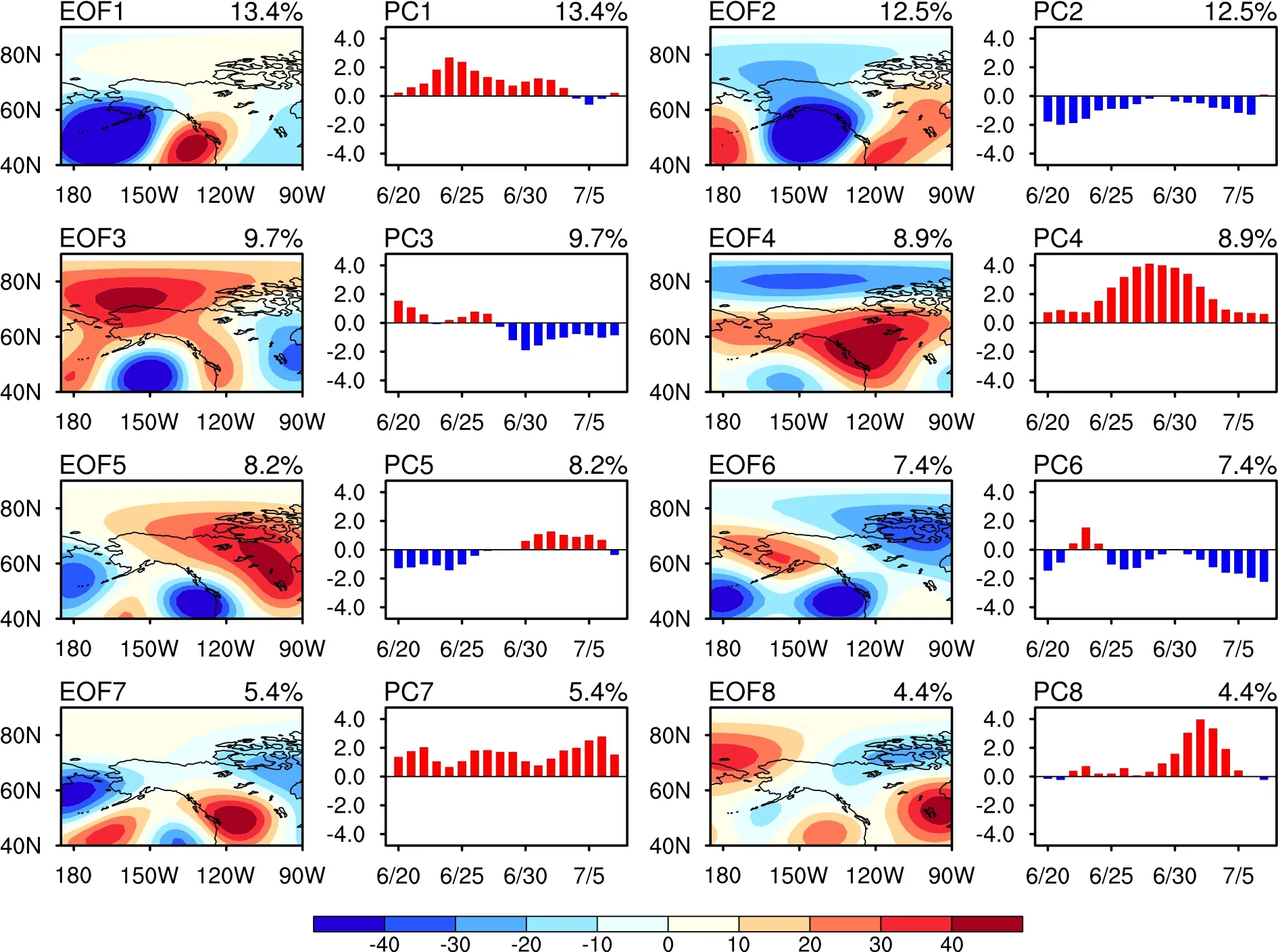
Fig.2.Eight leading empirical orthogonal function (EOF) modes (units: gpm).The EOF analysis is performed by using daily 300-hPa geopotential height in the region of 40°-90°N, 175°E-90°W during June-July from 1979-2021.Their corresponding principal component (PC) time series are shown from 20 June 2021 to 7 July 2021.The percentages of variance explained by EOF modes are given in the upper right corner.

The indices of these three patterns during late June and early July of 2021 are a testament to their roles in the formation and development of the western North America heatwave.The North Pacific pattern index peaked on 24 June,indicating that the role of the North Pacific pattern is to initial-ize and develop the heat dome.The Arctic-Pacific-Canada pattern index shows a positive value on 20 June and a maximum on 28 June.These relative timeframes imply that the Arctic-Pacific-Canada pattern is important in the development and mature phases of the western North America heatwave.The North America pattern index attains a maximum on 2 July,which suggests that the North America pattern coincides with the decay and eastward movement of the heat dome.Compared with historical records, the averaged North Pacific pattern index in late June of 2021 was the third highest since 1979, whereas the averaged Arctic-Pacific-Canada pattern index and the averaged North America pattern index in late June of 2021 were both record-breaking since 1979(Fig.5), again suggesting that the heat dome in western North America is associated with these three patterns.

Fig.3.Regressed daily surface air temperature anomalies (shading; units: °C) onto the corresponding PC time series of eight leading EOF modes during June-July from 1979-2021.The dotted areas denote statistical significance at the 95% confidence level.

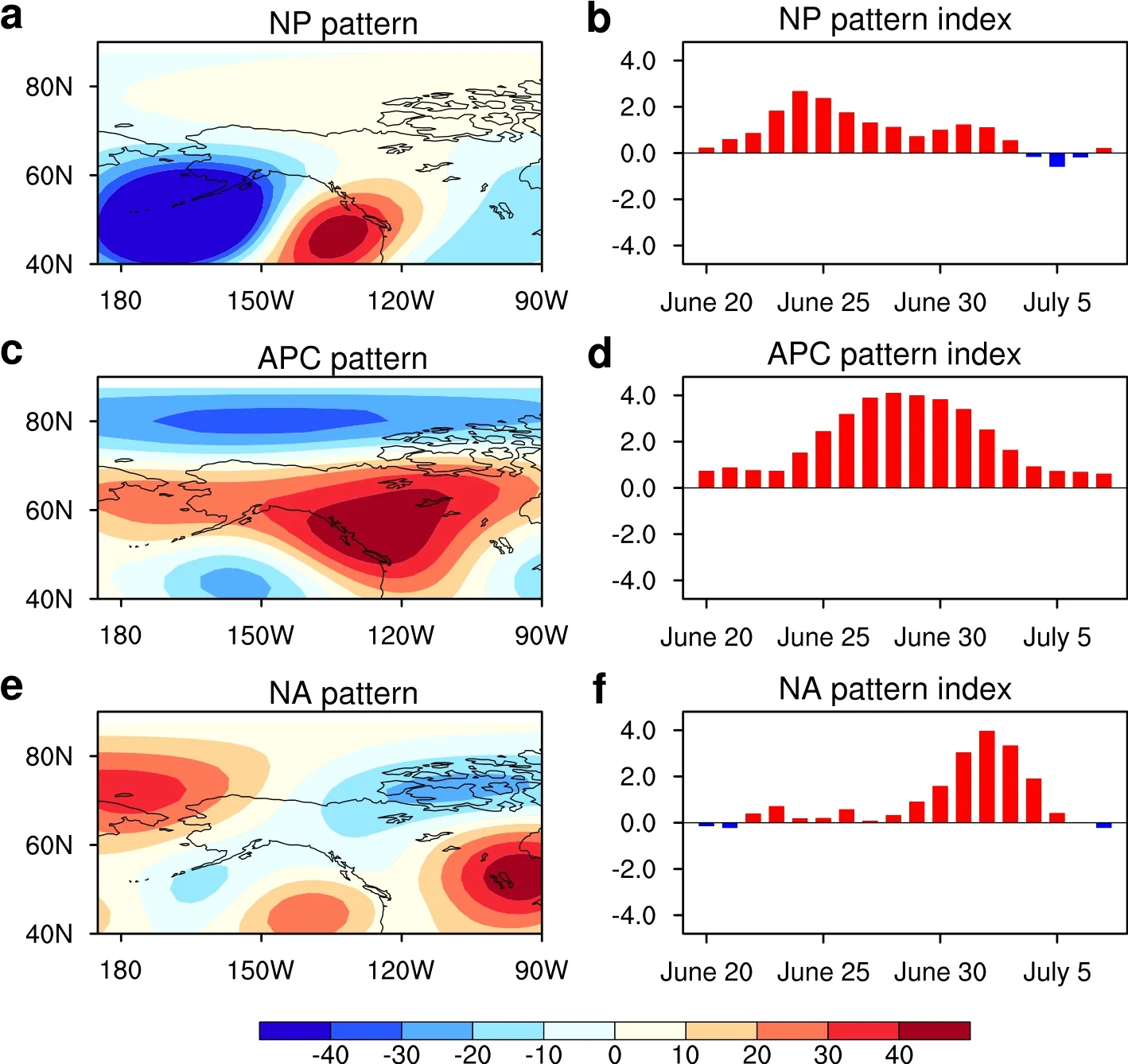
Fig.4.Three atmospheric patterns associated with the heatwave in western North America.(a,b) Spatial distribution of the North Pacific (NP) pattern (units: gpm) and the NP pattern index from 20 June to 7 July 2021.The NP pattern is obtained as the EOF1 mode of daily 300-hPa geopotential height anomalies in the region of 40°-90°N, 175°E-90°W from June-July from 1979 to 2021, whereas the NP pattern index is the PC1 time series.Panels (c, d) are similar to(a, b) but for the Arctic-Pacific-Canada (APC) pattern, which is obtained as the EOF4 mode.Panels (e, f) are similar to (a, b) but for the North America (NA) pattern, which is obtained as the EOF8 mode.

The common feature of these three patterns is that the positive geopotential height anomalies near the dome are accompanied by the remote negative geopotential height anomalies in the North Pacific and Arctic.We use atmospheric wave activity flux (Takaya and Nakamura, 2001; Li et al., 2019) to demonstrate the contributions of the negative poles to the heat dome.For the North Pacific pattern, a wave train is emanating from the North Pacific, suggesting that the negative geopotential height anomalies in the North Pacific enhance the positive geopotential height anomalies west of North America (Fig.6a).For the Arctic-Pacific-Canada pattern, both the negative geopotential height anomalies in the Arctic and North Pacific increase the positive geopotential height anomalies in Canada (Fig.6b), contributing to a strong anticyclone and extreme heatwave.During the decaying phase of the North America pattern, the negative geopotential height anomalies to the north are also emanating wave activity flux southward toward the positive geopotential height anomalies (Fig.6c).We also calculate atmospheric wave sources and sinks (the contours in Fig.6) which are described as the divergence of atmospheric wave activity flux.It is found that positive 300-hPa geopotential height anomalies are located in the downstream region of the atmospheric wave sink, suggesting that atmospheric wave activities associated with three atmospheric teleconnection patterns contributed to the positive 300-hPa geopotential height anomalies and led to the heatwave in western North America.

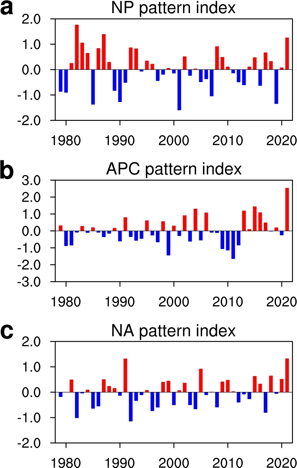
Fig.5.Time series of the NP, APC, and NA pattern indices averaged from 22 June to 4 July over the period 1979-2021.

3.2.Reconstruction of the heatwave

We have shown that the three modes of the NP, APC,and NA patterns can explain the heatwave that occurred in western North America from late June to early July of 2021.The next question is whether the heatwave in western North America can be reconstructed using these three atmospheric circulation patterns.Here, we simply use these three patterns to reconstruct the 300-hPa geopotential height and surface air temperature anomalies based on the extreme fitting method introduced in section 2.5.As shown in Fig.7, both the reconstructed geopotential height and temperature anomalies well resemble the observed distributions, again indicating that the three atmospheric circulation patterns are responsible for the western North America heatwave that occurred in late June of 2021.However, the amplitude of the reconstructed heatwave is smaller than the observed one.This implies that something else is also important for the western North America heatwave in addition to the three atmospheric circulation patterns.

3.3.Contribution of global warming

What is the contribution of global warming to this heatwave in western North America? The answer to this question requires the assistance of numerical model experiments.Fortunately, the Coupled Model Intercomparison Project Phase 6(CMIP6) includes a part of the Detection and Attribution Model Intercomparison Project (DAMIP).DAMIP contains different types of model experiments driven by various forcings, such as well-mixed greenhouse-gas-only (GHG) historical simulations, anthropogenic-aerosol-only (AER) historical simulations, and natural-only (NAT) historical simulations(Gillett et al., 2016; Seong et al., 2021).Since CMIP6 models are not designed to simulate a particular heatwave event, it is not surprising that these model outputs do not well reproduce the western North America heatwave that occurred in late June of 2021 (Fig.8).However, Gessner et al.(2021)and Fischer et al.(2021) used a single coupled model of the Community Earth System Model (CESM) to perform the ensemble experiments based on different initial conditions.They showed that the CESM could simulate exceptional heatwaves in central North America in 1995 and Europe in 2003.

Here, we use CMIP6 DAMIP model experiments to investigate the long-term causes of the average daily maximum temperature (Tmax) in the region of 40°-60°N, 100°-130°W.Figure 9 shows the observations, CMIP6 historical simulations, and CMIP6 model projections under global warming for the Shared Socioeconomic Pathways scenario(SSP2-4.5).The observed Tmaxanomaly from 15 June to 15 July 15 during 1951-2021 exhibits an upward trend of 0.22°C per decade with large fluctuations (OBS, black line).The simulated Tmaxanomaly from all external forcing (ALL)during 1951-2014 also shows an increasing trend of 0.30°C per decade, but the fluctuation is smaller than observations(red line).Compared with the ALL case, the GHG-induced Tmaxanomaly change shows an upward trend of 0.30°C per decade (purple line).In contrast, the AER contribution to the change of Tmaxanomaly is negative, with a trend of-0.013°C per decade (green line).The NAT forcing contributes little to the Tmaxanomaly with a trend of -0.018°C per decade (blue line).The characteristics of the Tmaxanomaly changes with different external forcing under the SSP2-4.5 scenario are similar to those in historical periods.The Tmaxanomaly under ALL and GHG forcings shows an increasing trend, while the Tmaxanomaly under NAT and AER forcings fails to show a trend in the future.

The present Tmaxanomaly changes from 15 June to 15 July between the periods of 2011-20 and 1961-90 are shown in Fig.9b.The black dashed line represents the change of the observed Tmaxanomaly.The increase in the Tmaxanomalies from ALL and GHG forcing simulations are larger than observations, while the changes from NAT and AER forcing are small.Similarly, the future Tmaxanomaly changes of different external forcing simulations between the periods of 2091-2100 and 2011-20 are displayed in Fig.9c.The increase of Tmaxanomaly from ALL and GHG forcing simulations are close to 3.2°C and 2.5°C, much higher than the increase from NAT and AER forcing simulations.These suggest that the increase in greenhouse gas concentration is a main reason for the increase of Tmaxboth inthe present and future.This is consistent with the results of Philip et al.(2022).They concluded that the occurrence of a heatwave of the intensity experienced in western North America would have been virtually impossible without humancaused climate change.The spatial distributions of the present and future Tmaxanomaly changes are relatively uniform, but the maximum changes are located between 40°-45°N (Figs.9d and 9e).

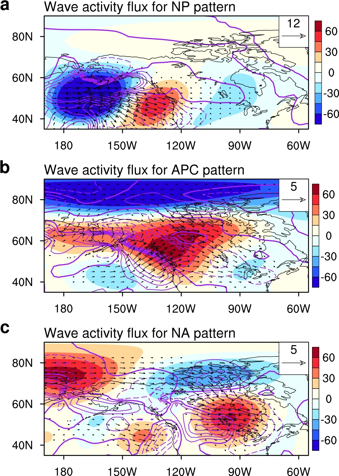
Fig.6.Atmospheric wave activity fluxes associated with three modes.Panel(a) shows the regressed daily 300-hPa geopotential height anomalies(shading; units: gpm) onto the North Pacific (NP) pattern index, the atmospheric wave activity flux (vectors; units: m2 s-2), and atmospheric wave sources and sinks (divergence of atmospheric wave activity flux; purple contour, units: m s-2) associated with the NP pattern.Panels (b, c) are similar to (a), but for the Arctic-Pacific-Canada (APC) pattern and the North America (NA) pattern, respectively.

Additionally, we show the probability density functions(PDFs) of the Tmaxanomalies in western North America from 15 June to 15 July for 1951-2021 from the observations(Fig.10) (Stott et al., 2004; Fischer and Knutti, 2015).The PDFs are estimated by the kernel smoothing function.Similarly, the PDFs of the Tmaxanomalies from ALL (HIST),NAT (HIST), GHG (HIST), and AER (HIST) simulations during 1951-2020 and ALL (SSP245), NAT (SSP245), GHG(SSP245), and AER (SSP245) simulations during 2021-2100 of CMIP6 are also shown in Fig.10.Based on the two-sided Kolmogorov test, the observed and ALL simulated PDFs during 1951-2020 are not significantly different at the 0.05 level, which means that CMIP6 models can effectively simulate the PDFs of the Tmaxanomalies in western North America during 1951-2020.The vertical black dashed line in Fig.10 shows the observed 2021 Tmaxanomalies in western North America.The areas enclosed by the dashed line and the PDFs distribution represent the probabilities of this kind of extreme event under different external forcings (Table 2).There is a clear rightward shift of the PDFsof the Tmaxanomalies from the ALL (HIST) and GHG(HIST) simulations compared with the NAT (HIST) and AER (HIST) simulations.It is suggested that human influences, like increased greenhouse gas concentration, have increased the probability of warm events.The PDFs from ALL and GHG simulations during 2021-2100 show a more rightward shift than those during 1951-2020.The probability of this extreme event increases by 32.18% under the ALL simulation and 20.42% under the GHG simulation in the future.The probability ratio and the fraction of attributable risk of an extreme event, like the observed 2021 heatwave, are 6.14 and 0.84 during 1951-2020 (171.54 and 0.99 during 2021-2100) (see Table 2 for 95% confidence intervals).This also indicates that human influences have increased the probability of an extreme event, like the 2021 heatwave.

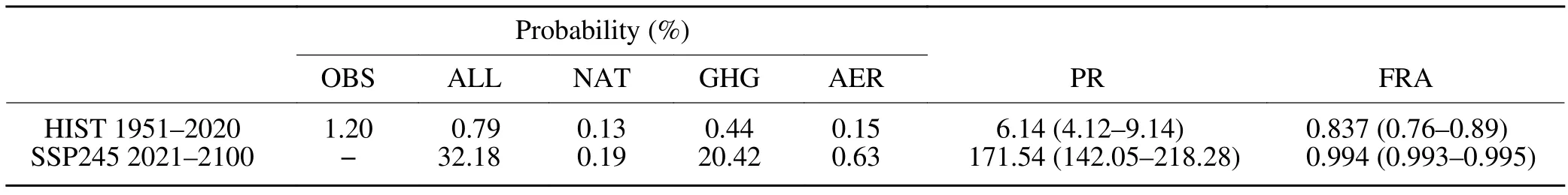
Table 2.The probabilities of an extreme event like the observed 2021 heatwave under different external forcing simulations.The probability ratio (PR) and the fraction of attributable risk (FAR) with 95% confidence intervals of extreme events, like the observed 2021 heatwave.

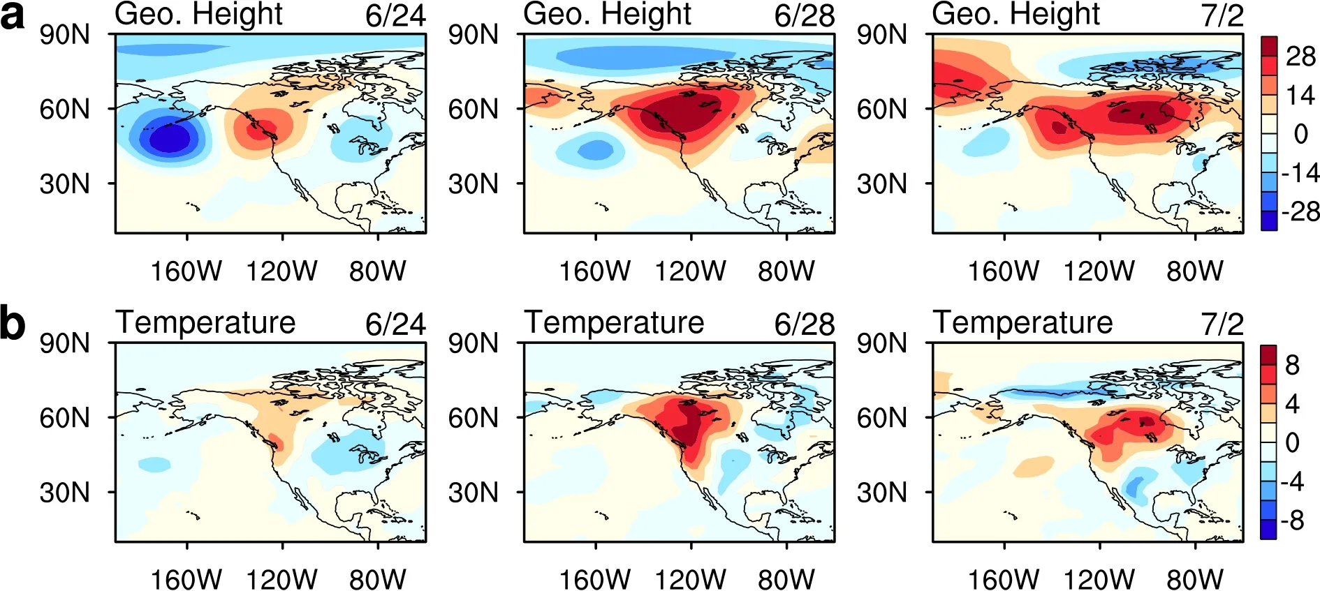
Fig.7.Reconstructed Pacific Northwest heatwave from 24 June to 2 July 2021.(a) Reconstructed daily 300-hPa geopotential height anomalies (shading; units: 10 gpm) from 24 June to 2 July 2021 by using the North Pacific, Arctic-Pacific-Canada,and North America pattern indices.Panel (b) is similar to (a) but for reconstructed surface air temperature anomalies at the sigma-995 level (shading; units: °C).

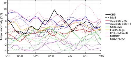
Fig.8.The time series of Tmax anomalies (°C) in western North America from 15 June to 15 July 2021 from observations (OBS, solid black line), 17 simulations of 7 CMIP6 climate models, and the multi-model ensemble mean (MME, black dash line).Different curves in the same color represent different members of the same model.

4.Discussion and summary

The Arctic polar vortex is a cap of rotating air that is usually centered on the North Pole.It is suggested that weakening and splitting of the stratospheric polar vortex, which are associated with a wavy pattern of the jet stream in the troposphere, can result in extreme weather events in the mid-latitudes (e.g., Kim et al., 2014; Peings and Magnusdottir,2014; Nakamura et al., 2015; Overland, 2021; Wang et al.,2021).Here, we analyze the geopotential height field at 100-hPa prior to the heatwave event.As shown in Fig.11,an Arctic polar vortex split event occurred prior to the heat-wave on 17 June, with one low-pressure center moving southward into the North Pacific (Overland, 2021).This low-pressure center strengthened until 24 June and contributed to the positive phase of the NP pattern.This suggests that the polar vortex split event may be related to the NP pattern identified in this paper and may be responsible for initializing and developing the heat dome.However, the polar vortex split event can not explain the mature and decaying phases of the heatwave since the low-pressure center was weak on 28 June and 2 July.It should be noted that the polar vortexwas re-established on 28 June, whereas the polar vortex moved eastward on 2 July.The re-establishment and movement of the polar vortex coincided with the evolution of the APC pattern and the NA pattern.The influence of the polar vortex (associated with the Arctic sea ice loss and global warming) on extreme weather events is an interesting topic to be further studied.

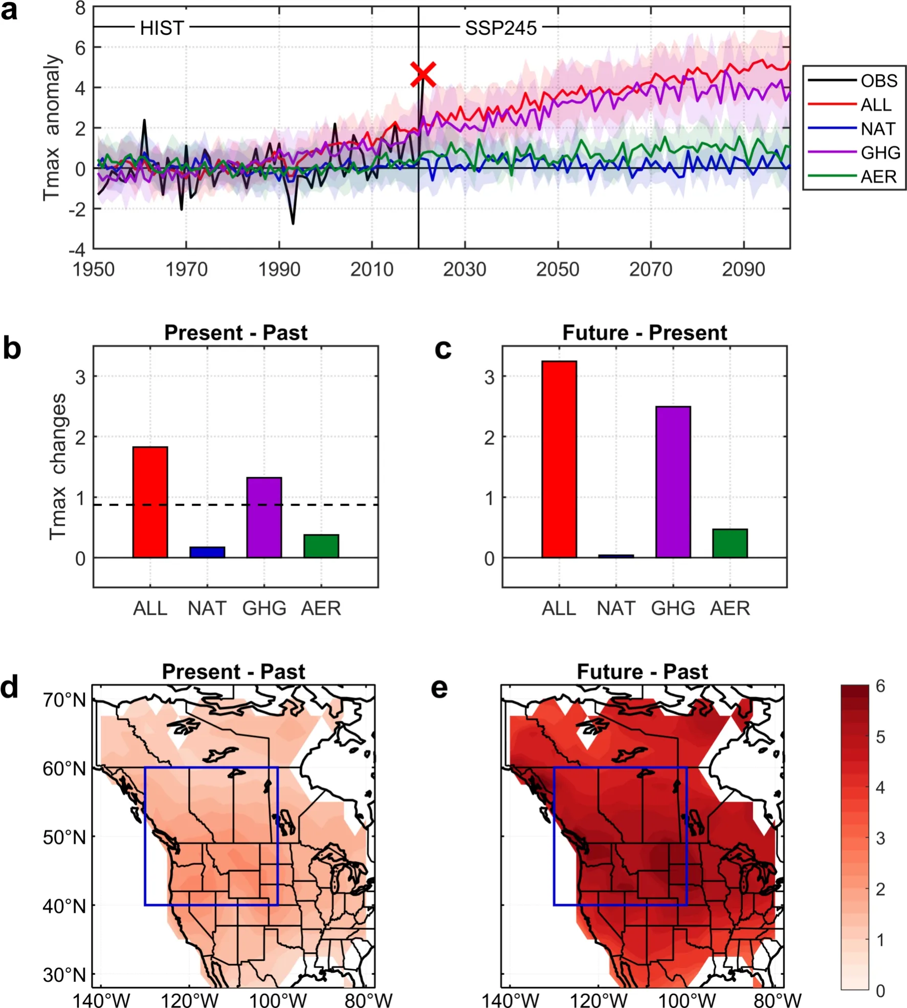
Fig.9.Tmax anomaly from observations and model simulations.(a) The time series of Tmax anomaly (°C) in western North America from 15 June to 15 July based on 1951-2021 observations and CMIP6 simulations during 1951-2020(HIST) and 2021-2100 (SSP245).The black line represents the observations (OBS) from the GHCND dataset.The red cross represents the observed 2021 Tmax anomalies.The red, blue, purple, and green lines represent ALL, NAT,GHG, and AER forcings, respectively.The shading represents one standard deviation across all models.NAT, GHG,and AER forcings in the SSP245 period have only two models (CanESM5 and MIROC6).(b) The present (2011-20)changes in the Tmax anomaly based on different external forcing relative to the past period (1961-90).The black dashed line represents the change of the observed Tmax anomaly.(c) The future (2091-2100) changes of Tmax anomaly based on different external forcing relative to the present period (2011-20).(d) The spatial distribution of Tmax anomaly based on ALL forcing in the present (2011-20) relative to the past period (1961-90).(e) Similar to (d),but for the future (2091-2100) period relative to the past period (1961-90).

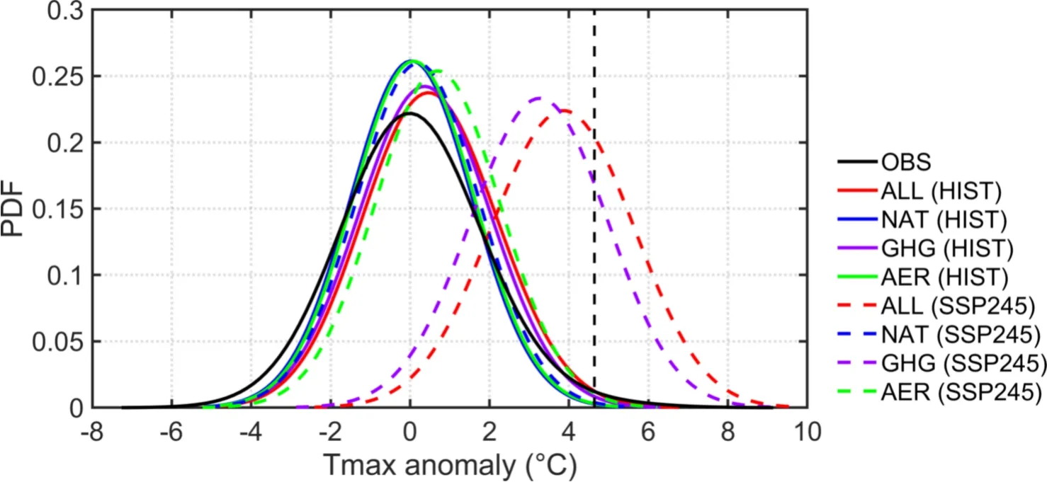
Fig.10.Probability density functions (PDFs) of Tmax anomalies (relative to 1961-90) in western North America from 15 June to 15 July for the observations and CMIP6 simulations.The black line represents the Tmax anomalies from the GHCND observation during 1951-2021.The red,blue, purple, and green lines represent the Tmax anomalies from ALL, NAT, GHG, and AER forcing during 1951-2020 (solid line, HIST) and 2021-2100 (dash line, SSP245).The vertical black dashed line is the observed Tmax anomalies of the 2021 extreme event in western North America.

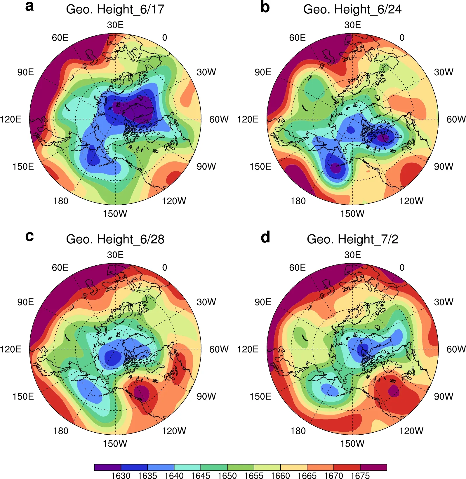
Fig.11.Geopotential height at 100-hPa (units: 10 gpm) on (a) 17 June 2021, (b) 24 June 2021, (c) 28 June 2021, and (d) 2 July 2021.

Another issue is the possible linkage of these three patterns with the oceans.To see whether the three atmospheric circulation patterns are related to the oceans, we regress SST anomalies onto the NP, APC, and NA pattern indices from 22 June-4 July for the period 1982-2021 (not shown).All three patterns fail to show significant regressed SST signals in the tropical oceans.The SST anomalies from 22 June to 4 July 2021 did not show significant signals in the tropical oceans either.These may indicate that tropical climate variability such as ENSO has little to do with the heatwave in western North America.However, the three patterns do show some relationships with the North Pacific SSTs,and the SST anomalies in the North Pacific from 22 June to 4 July 2021 were positive, suggesting that these positive SST anomalies may affect weather in North America.Atmospheric response to mid-latitude SST anomalies is a longstanding and perplexing problem (Folland et al., 2009; Lau and Nath, 2012; Zhou, 2019) and deserves further study.

This paper uses observational data to identify three atmospheric circulation patterns associated with the western North America heatwave that occurred in late June of 2021.It is shown that the North Pacific and Arctic-Pacific-Canada patterns co-occur with the development and mature phases of the heatwave in western North America, whereas the North America pattern coincides with the decay and eastward movement of the heatwave in western North America.CMIP6 climate models show that greenhouse gases are a main reason for the long-term increase of the average daily maximum temperature in the region of western North America during the past and into the future.However, CMIP6 climate models are not designed to simulate a specific heatwave event in western North America.The probability of an extreme heatwave event increases by 32.18% under the ALL simulation and 20.42% under the GHG simulation in the future.It is likely that global warming associated with an increase in greenhouse gases influences these three atmospheric circulation pattern variabilities, thus affecting the occurrence of heatwaves in western North America.The regional and short-timescale variations in climate, such as heatwaves, deserve more attention and study.

Acknowledgements.This study is supported by the Key Special Project for Introduced Talents Team of Southern Marine Science and Engineering Guangdong Laboratory (Guangzhou)(GML2019ZD0306), National Natural Science Foundation of China (Grant Nos.41731173 and 42192564), National Key R&D Program of China (2019YFA0606701), Strategic Priority Research Program of Chinese Academy of Sciences (XDB42000000 and XDA20060502), Innovation Academy of South China Sea Ecology and Environmental Engineering, Chinese Academy of Sciences(ISEE2021ZD01), Independent Research Project Program of State Key Laboratory of Tropical Oceanography (Grand No.LTOZZ2004), and Leading Talents of Guangdong Province Program.The numerical simulations were supported by the High Performance Computing Division in the South China Sea Institute of Oceanology.

Data availability.All data in the main text or the Supplementary information and Methods are available.In the main text, NCEP/NCAR reanalysis data are available at https://psl.noaa.gov/data/gridded/data.ncep.reanalysis.html.GHCND observation data are available at ftp://ftp.ncdc.noaa.gov/pub/data/ghcn/daily/grid/.CMIP6 model data are available at https://esgf-node.llnl.gov/projects/cmip6/.The NOAA OISST high-resolution dataset, which is v2.0 over 1982-2015 and v2.1 over 2016-21, is available at https://psl.noaa.gov/data/gridded/data.noaa.oisst.v2.highres.html.

Open AccessThis article is licensed under a Creative Commons Attribution 4.0 International License, which permits use, sharing,adaptation, distribution and reproduction in any medium or format,as long as you give appropriate credit to the original author(s) and the source, provide a link to the Creative Commons licence, and indicate if changes were made.The images or other third party material in this article are included in the article’s Creative Commons licence, unless indicated otherwise in a credit line to the material.If material is not included in the article’s Creative Commons licence and your intended use is not permitted by statutory regulation or exceeds the permitted use, you will need to obtain permission directly from the copyright holder.To view a copy of this licence,visit http://creativecommons.org/licenses/by/4.0/.