Magnetohydrodynamic Kelvin–Helmholtz instability for finite-thickness fluid layers

Hong-Hao Dai(戴鸿昊) Miao-Hua Xu(徐妙华) Hong-Yu Guo(郭宏宇)Ying-Jun Li(李英骏) and Jie Zhang(张杰)

1State Key Laboratory for Geomechanics and Deep Underground Engineering,China University of Mining and Technology,Beijing 100083,China

2School of Science,China University of Mining and Technology,Beijing 100083,China

3Double-cone Ignition(DCI)Joint Team,China University of Mining and Technology,Beijing 100083,China

4Double-cone Ignition(DCI)Joint Team,Beijing National Laboratory for Condensed Matter Physics,Institute of Physics,Chinese Academy of Sciences,Beijing 100190,China

Keywords: finite-thickness,Kelvin–Helmholtz instability,magnetohydrodynamic,inertial confinement fusion

1. Introduction

Hydrodynamic instabilities at the interface of two fluids with different densities are concerned in high energy density physics (HEDP). The Kelvin–Helmholtz instability (KHI) is a ubiquitous issue in HEDP. KHI arises when there is a difference in the fluids’s velocities parallel to the interface of the two fluids, causing fluids near the interface to curl and tumble. KHI is widely found in nature, such as the interaction of the solar wind and the geomagnetic field,[1]the meteorological change,[2]and so on. The study of KHI can also provide theoretical guidance for experimental works of inertial confinement fusion(ICF)[3]and magnetic confinement fusion(MCF).[4]

Chandrasekhar studied the classical KHI and obtained the analytic formula of linear growth rate and frequency. Weakly nonlinear analysis of the KHI of fluids under incompressible conditions was analyzed by Wanget al.[6–8]The results agreed well with the numerical simulation. Wanget al.[9,10]also found that the combined effect of density and velocity gradients stabilizes the KHI in most cases. When the fluids were affected by magnetic fields,Chandrasekhar[5]showed that the development of the KHI would be suppressed by the uniform magnetic field acting parallel to the direction of streaming.Grattonet al.[11]studied the effect of large perturbation wavelengths on the magnetic fluid KHI by solving the MHD control equations using a confinable model. The results show that when the direction and magnitude of the magnetic field are constant, the KHI does not exist in the long boundary layer.Sharma and Srivastava[12]investigated the effect of rotating and tilting magnetic fields on the KHI and derived the dispersion relation for equal density and different velocities. They found that even in the presence of rotation,the magnetic field still has a stabilizing effect. Zhaoet al.[13]indicated that KHI at the interface of incompressible fluids with continuous profiles was suppressed under the effect of the magnetic field in an infinite two-dimensional plane,but the magnetic field gradient scale length effect increased the linear growth of KHI.All these works emphasized that the magnetic field decreases the growth rate of KHI under specific conditions.

We should notice that KHI often occurs at the interface in the late stages of development of Rayleigh–Taylor instability(RTI)or Richtmyer–Meshkov instability(RMI),[14]the generation of strong shear flow excites the KHI leading to smallscale mixing of fluids and aggravates the nonlinear development of RTI or RMI.[15]For example,the process of a heavier fluid intruding into a less dense fluid to form a“spike”under the action of gravitational field will excite the KHI,the“spike”is fluids with a finite thickness,and the effect of its thickness on the KHI cannot be ignored. Recently, experimental campaign of double-cone ignition scheme for ICF led by Zhang[16]has been carried out. In this experiment,the KHI is excited at the interface between the cone-target wall made of metal Au and the plasma fuel due to the tangential velocity difference.The Au metal can be mixed into the target port via the curling effect of the KHI, causing a decrease in the density and temperature of the fuel, which may lead to ignition failure. It is believed that coating a thin film layer on the target wall reduces the growth rate of the KHI.But no one has given a relevant theoretical analysis of the KHI that may be excited inside this thin film layer (coating). Our finite thickness model may provide some theoretical references to this problem. Thus, we would like to learn more about the development of the KHI problem in fluids with finite thickness. In combination with the magnetic field effects, in this article, assuming the magnetic field acting parallel to the direction of the fluid’s velocity, we investigate the linear growth rate of KHI at the interface with velocity and density discontinuity, of two finite-thickness superimposed fluid layers,and each of the fluid layers has got an arbitrary thickness. We study the effect of fluid thickness on KHI with and without a magnetic field.

This paper is organized as follows: In Section 2, we describe the theoretical model and briefly discuss the eigenvalue problem of the KHI for fluids with finite thickness. We derive the equation for solving the eigenvalue, and the correctness of the equation is verified. Section 3 displays that the linear growth rate has been obtained by a numerical method, which is compared with the analytical formula. In Section 4,we discuss the effect of the fluid thickness and the magnetic field on the linear growth of KHI in detail. The major results and some conclusions are given in Section 5.

2. Theoretical model

The ideal incompressible fluid is considered in a magnetic field ignoring the surface tension,viscosity,rotational and heat transfer. We can use ideal MHD equations to describe the behavior of incompressible fluids. In a Cartesian coordinate system,the ideal MHD equations can be written as

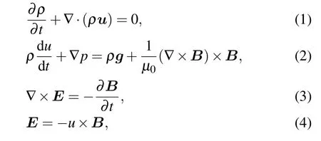
whereρ,p,u,g,E,B,andµ0are the density,thermal pressure, velocity, gravitational acceleration, electric field intensity,magnetic flux density,and magnetic permeability,respectively. The physical quantity of hydrodynamics can be expressed as the sum of zero order equilibrium quantity and firstorder disturbance, thus we obtainu=u0+u1,p=p0+p1,ρ=ρ0+ρ1,B=B0+B1. Combined with our specific model, the velocity and magnetic field can be further expressed in the form of vector, which can be written asu=u0+u1=u0xi+u1xi+u1yj,B=B0+B1=B0xi+B1xi+B1yj.There is another equation ∇·u=0,which is the assumption of incompressible fluids,can be written as∂u1x/∂x+∂u1y/∂y=0.

Substituting the rewritten physical quantities into Eqs. (1)–(4), along with the equation obtained from the assumption of incompressible fluids,the linearized equations are

The Fourier analysis is performed on the perturbed quantities as

this equation combined with appropriate boundary conditions forms an eigenvalue problem.

Now we consider two fluids distributed above and below the interface aty=0, and both of them have finite thickness.We assume that the velocity and density distribution of the fluid to be in the form of discontinuous,and the magnetic field acting parallel to the direction of the fluid’s velocity. We denote the physical quantities of the upper(lower)fluids by subscripts 1(2).For example,the fluid density above the interface isρ1,the fluid density below isρ2,the thickness of the upper fluid ish1, the thickness of the lower fluid ish2and so on.Now, the specific expressions of the magnetic field and the fluid’s density, velocity under the finite thickness model are given as follows:

The density and velocity of the fluid itself are discontinuous, while the external magnetic field is continuous with a transition layer,whereU1(U2),ρ1(ρ2),are velocity and density above(below)the interface in thexdirection,respectively.B1(B2)represents magnetic field intensity in the upper(lower)fluids,andLBis the thickness of the magnetic field transition layer, ∆B=B1−B2. We use this form of the magnetic field distribution expression because we consider the boundary conditions where the magnetic fields vanish at the boundaries of the fluids. Also the magnetic field curve in this form is close to the magnetic field distribution in experiments.

It is worth noting that the zeroth order fields must satisfy the MHD equilibrium conditions. Without the influence of gravity field(g=0),theydependence of the kinetic(fluid)pressurep0(y)and the magnetic fieldB0(y)should satisfy the equilibrium condition which means that the zeroth order fields satisfy the equilibrium conditions at the interfacey=0.

We assume the approximate eigenfunction as follows:[17]

Ash1k=h2k →∞, the magnetic field integral on the right-hand side of Eq. (12) is then extended to the infinite space case. After simplifying our magnetic field integral,we can find that it agrees with the magnetic field integral in Eq.(17)in Ref.[13].

Ash1k=h2k →∞, withU1=U2=0,LB=0,g/=0,one can see our problem degenerates to classical Rayleigh–Taylor instability (RTI) problem in discontinuous magnetic field.LetU1=U2=0,LB=0,solving the characteristic equation Eq.(21),we obtain

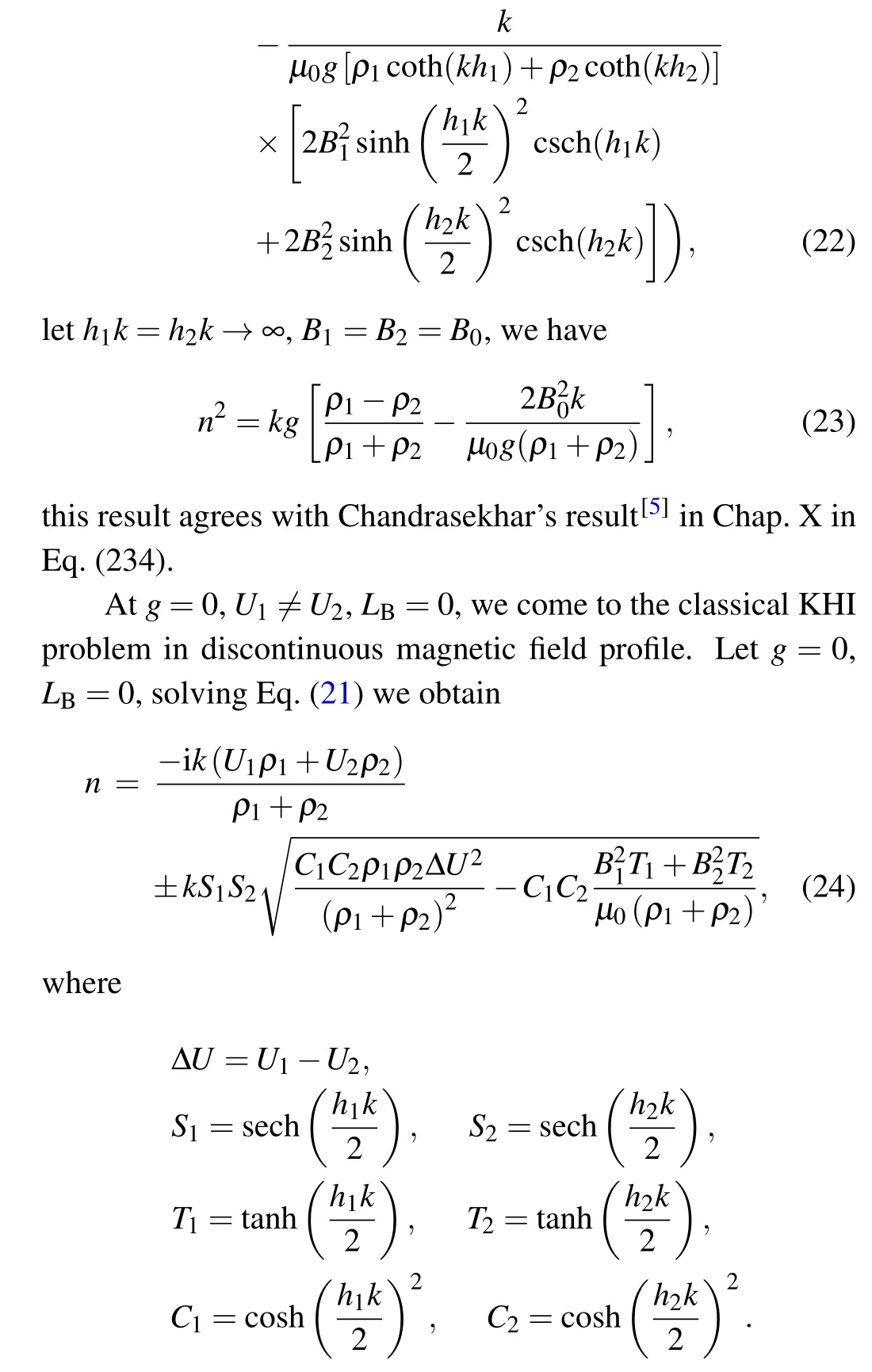
Leth1k=h2k →∞,B1=B2=B0,equation(24)can be simplified as

this equation agrees with Eq. (204) in Chap. XI in Chandrasekhar’s work[5]in the absence of the gravitational acceleration(g=0).

3. Numerical methods

3.1. Brief introduction

The second-order differential equation(12)about the perturbed velocity～vcan be rewritten as

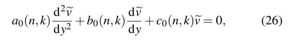
wherea0(n,k),b0(n,k),c0(n,k)are the coefficients of the corresponding terms of the second-order ODE (Eq. (12)). The first-and second-order derivatives can be solved by the central difference scheme with a second-order precision. The computing zone ranges from 0 toj+1 with step lengthh,and the boundary condition is ～v0=～vj+1=0. Let Eq. (26) divide bya0(n,k),then with nodej,the differential equation will be

where～bj=b0/a0,～cj=c0/a0. In matrix form,M(n,k)～V=0 represents Eq.(27),where～V=(～v1,～v2,...,～vJ)Tis an eigencolumn withJcomponents,and

is aJ×Jtridiagonal matrix. If the linear system of Eq. (27)has nonzero solutions, the determinant value of the matrixMmust be zero. In our numerical calculation, we find the nonzero roots of|M(n,k)| = 0 by the Hooke–Jeeves (HJ)searching method with applying an iteration method to calculate the determinant. We use this method to obtain the eigenvalue, and compare the numerical results with analytical formulas.

Generally speaking,we can findJroots of dispersion relation on the number of perturbed wavesnl(l=1,2,3,...,J)from the equations,each root or eigenvalue will associate with an eigenvector～Vl=(～v0,～v1,～v2,...,～vJ,～vJ+1),called thel-th perturbed mode. The eigenvalues are arranged in order of magnitude:n1≥n2≥n3≥···≥nJ. The real perturbation will be a linear superposition of all the possible modes. We only take the maximum eigenvalue, called the lowest or the first-order mode, as the estimation of the upper limit of the growth rate.In our numerical method,we find the maximum eigenvalue in the complex plane by the Hooke–Jeeves searching method.

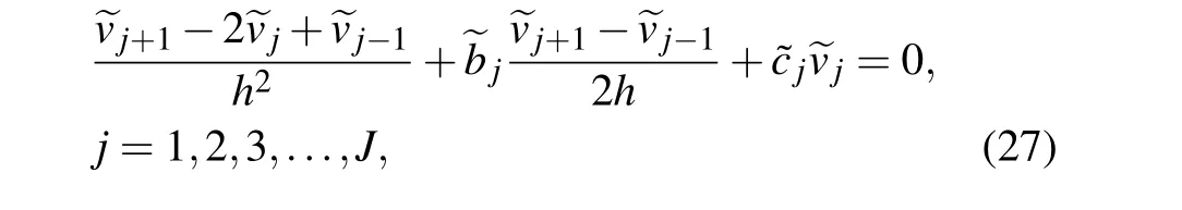
We setρ1=8,ρ2=1,U1=1,U2=−1,h2=1,k=1.Figure 1 shows the growth rate at different thicknesses of the upper fluidh1without the effect of the magnetic field. The black solid line represents the analytical growth rates results,and the red dots represent the numerical results. It is clear that the simulation results agree well with our analytic formula.

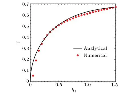
Fig. 1. The results of linear growth rate from our analytical formula and numerical simulation at different thicknesses of the upper fluid h1 without the magnetic field.

Taking magnetic field effects into consideration, the growth rate at differenth1is shown in Fig.2. The relevant parameters are:ρ1=8,ρ2=1,U1=1,U2=−1,h2=1,k=2,B0=0.5,µ0=1.As shown in Fig.2,for most of the numerical results,they agree with the analytical formula.There are some differences between the analytical growth rates and numerical results,while the errors are acceptable.

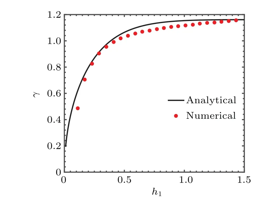
Fig. 2. The results of linear growth rate from our analytical formula and numerical simulation at different thicknesses of the upper fluid h1 with the magnetic field.

Fig. .3 The velocity distribution profile with Lu = λ/20π, λ/200π,λ/2000π. The value of the perturbed wavelength λ is 2π.

Since the perturbations is infinitely small values relative to the zero-order quantities, the absolute values of ～vis not that matter, only the distribution of ～vas perturbation profile is meaningful. Assumingλ=2π,Lρ=Lu=L, we plotted the distribution of ～v/～vmaxshown in Fig. 4. The black line is the analytic formula(～v/～vmaxin Eq.(16)),the lines in different styles represent the numerical results under differentL. Figure 4 presents that whenLis much smaller compared toλ,the numerical results for the distribution profile of ～vagree well with the analytical results, and this conclusion consists with our assumption.

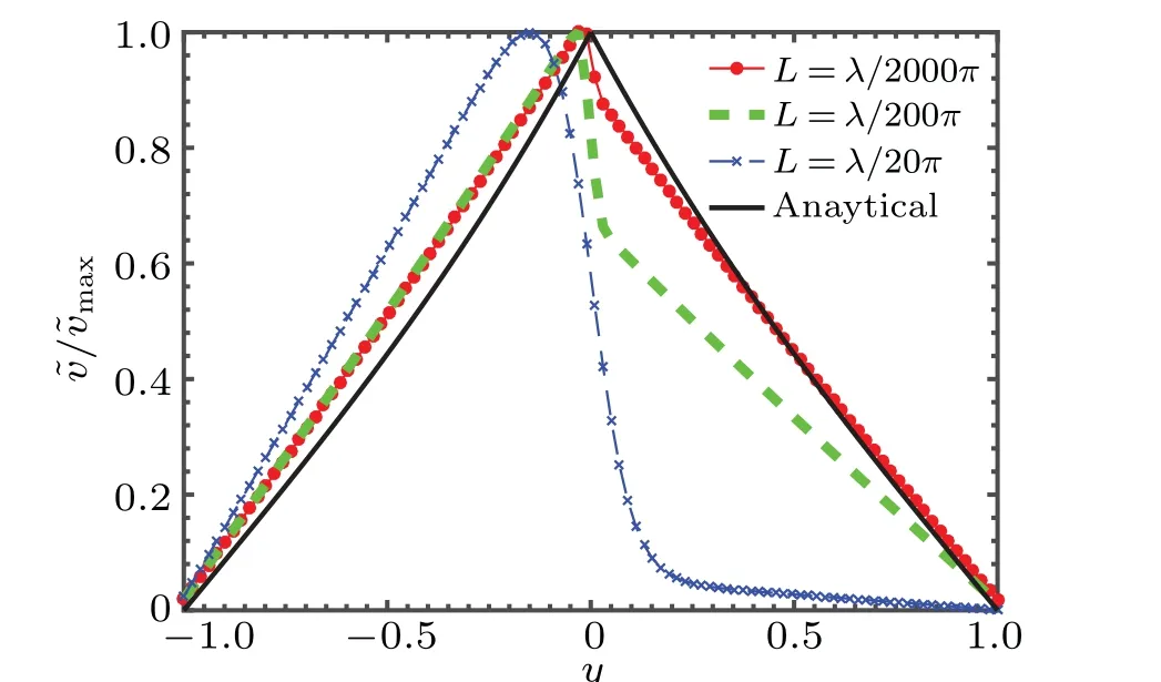
Fig. 4. The results of linear growth rate from our analytical formula and numerical simulation at different thicknesses of the upper fluid h1 without the magnetic field.

3.2. Accuracy of the numerical methods

The specific expressions of the velocityu0and densityρ0in our numerical method are[9]

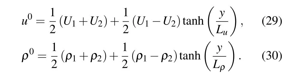
We use expressions of these forms to approximate the distribution ofu0andρ0in Eqs.(13)and(14). Since the density and velocity of the fluid are discontinuous in our article,LuandLρin Eqs.(29)and(30)must be very small. LetU1=1,U2=−1,we take Eq.(29)as an example. As shown in Fig.3,whenLuis much smaller compared toλ, the velocity distribution profile is more in line with the form of discontinuous distribution.

WhenLis much more smaller compared toλ, likeL=λ/2000π,the numerical solution should be more accurate theoretically. However, due to the accuracy of our numerical method and the limitations of derivative expressed by difference method at discontinuous interfaces, whenLis of such a small or smaller order of magnitude,the numerical results instead differ significantly from the analytical solution. Therefore, in our numerical method, in the order of magnitude ofL=λ/200π,the numerical results are in good agreement with the analytical results. As can be seen in Fig. 3, we argue that forL=λ/200π, the density and velocity gradient scale lengthsLis small enough for the perturbation wavelengthλso that the distribution ofu0andρ0at the interface can be considered as discontinuous in the numerical method.

As we have mentioned before,the magnitude ofLrelative toλwill greatly affect the accuracy of our numerical solution. WhenLis very small relative toλ(e.g.,L=λ/2000πor smaller)or close toλ(e.g.,L=λ/20πor larger),the numerical growth rates differ significantly from the analytical results.As shown in Fig. 5, the dots in different styles represent the numerical results under differentL, the black line is the analytic formula. In the case ofL=λ/200π(purple square dots)orL=λ/20π(green star-shaped dots),the numerical growth rates differ from the analytical results. WhenLis smaller in this case,e.g.,L=λ/200πorL=λ/2000π, the differences between the numerical growth rates and the analytical results will be even greater, and some numerical results will be invalid. WhenL ≈5λ/200π,the numerical growth rates agree well with the analytical results,we consider this to be the appropriate value ofLthat makes the numerical solution more accurate in this case.

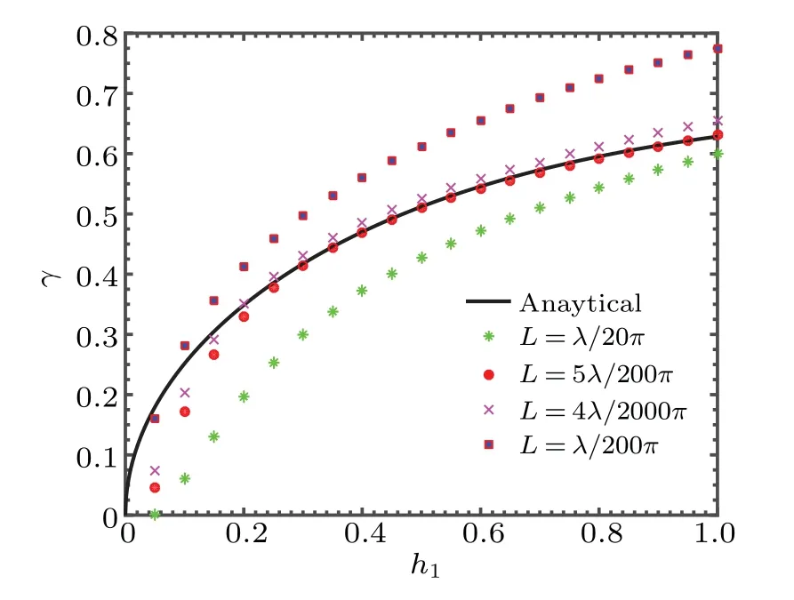
Fig. 5. The results of linear growth rate from our analytical formula and numerical simulation at different thicknesses of the upper fluid h1 without the magnetic field.

Based on the discussions above, we should consider the limitations of the numerical method and the validity of the approximation in Eqs.(29)and(30)to choose the appropriateLρ(Lu)in order to make the numerical results more accurate.

4. Results and discussion

4.1. Without magnetic field

When the fluid is not influenced by the magnetic fields,we remove the magnetic field influence term from the righthand side of the characteristic equation, and we letg= 0,the linear growth rate of KHI with finite thickness is yielded(∆U=U1−U2)

When the thickness of the fluid above and below the interface are equal,that ish1=h2,obviously we have

Assuming thatρ1>ρ2,figure 6(a)shows the normalized linear growth rates at different dimensionless thicknessd1withd2=0.5, 0.8, 1.2, 1.5. The density and shear velocity of the upper(lower)fluids areρ1=8,U1=10(ρ2=1, U2=−10),and the wave numberk=1.As shown in Fig.6(a),for fixed dimensionless thickness of the upper fluidd1,the linear growth rate decreases with the dimensionless thickness of the lower fluidd2. Whend2is larger, the decrease ofγNbecomes less obvious.

Figure 6(b) displays that for fixed dimensionless thickness of the lower fluidd2, the normalized linear growth rate increases withd1. The relevant parameters arek=1,ρ1=8,ρ2=1,U1=10,U2=−10,withd1=0.5,0.8,1.2,1.5.Whend1is larger,the increase ofγNbecomes less obvious.

Whend1andd2are large enough, the normalized linear growth rateγNreaches a more stable value and no longer changes significantly with the growth ofd1andd2. We approximate this to be the case of semi-infinite fluid layers,and the linear growth rate under such condition can be extracted by solving the special case of Eq.(17)(i.e.,khi →∞,i=1,2).

Atρ1<ρ2,we swap the positions of the two-fluid layers,and the conclusions we draw remain unchanged since there is no influence of the external potential field. These results remind us that reducing the fluid thickness on the denser side or increasing the fluid thickness on the less dense side can both suppress the linear growth of KHI,and the lager the value ofd2(d1),the less obvious the decrease(increase)ofγN.

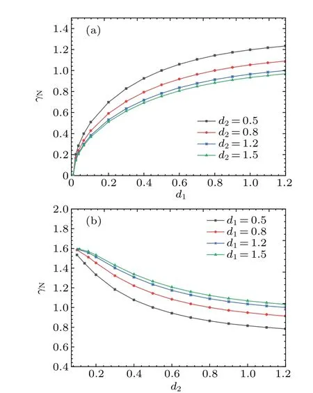
Fig.6.The normalized linear growth rate γN versus the dimensionless thickness of the upper fluid d1 (a) and the dimensionless thickness of the lower fluid d2 (b).

In the specific experimental scheme of double-cone ignition,multiple lasers are shot into the interior of the conical target.The laser incident will ablate the fuel,forming a compression effect to the inside of the cone target; it will also ablate the coating on the target wall,causing a change in the density distribution of the coating. As a result,the velocity difference effect will be visible at the coating and the KHI will be excited inside the coating. Letd1+d2=Dbe the total dimensionless thickness,and letd1=d,the normalized linear growth rate of KHI without magnetic field effect is

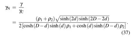
Since the density distribution of the coating varies in our practical problem, we only consider the case ofρ1/=ρ2. Ifρ1>ρ2, given the initial values ofρ1=8,ρ2=2,d=0.1,0.3,0.5,0.7,1,∆U=2,k=1,figure 7 shows the relationship between the dimensionless total thicknessDand the normalized linear growth rateγN.

As shown in Fig. 7,γNalways increases rapidly withDand reaches the maximum value, then decreases withDat a slower rate. The values ofDcorresponding to the maximum growth rate are related to the density ratioρ1/ρ2. This effect is more obvious for larger values ofd, but less obvious for larger values ofρ1/ρ2. During the decrease ofγN, the larger the value of the initial dimensionless thicknessdis,the more slowlyγNdecreases. This suggests that we should select the proper thickness of the coating to reduce the linear growth of KHI in the experiments. Ifρ1<ρ2,based on the symmetry of our model,the conclusion should be consistent.

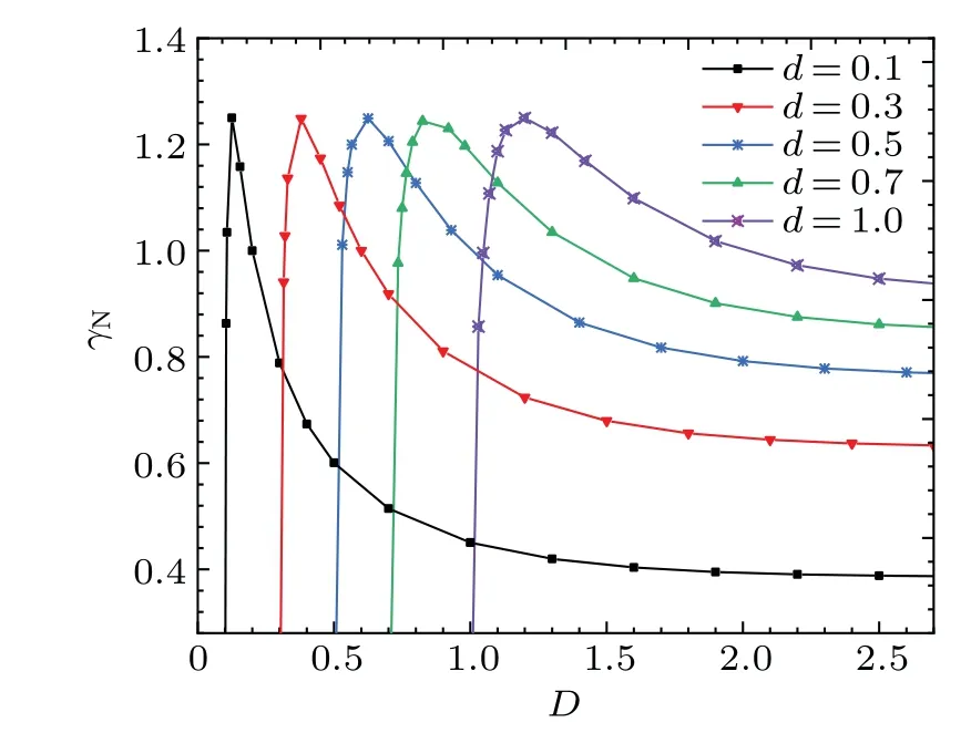
Fig.7. The normalized linear growth rate γN versus the dimensionless total thickness of the fluid D.

4.2. With external magnetic field

Next we will take the effect of the magnetic field into consideration. AtLB= 0,g= 0, we assume that upper fluid’s magnetic field intensity is equal to the lower one(i.e.,B1=B2=B0), we can obtain the normalized linear growth rate

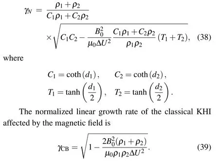
Atρ1>ρ2, the relationship between the magnetic field intensityB0andγNare shown in Figs.8(a)and 8(b).

It is found thatγNdecreases more slowly thanγCBas the magnetic field strengthB0increases. This suggests that a stronger magnetic field is needed to completely suppress the linear growth of the KHI when considering the thickness of the fluid. It can be seen from Fig.8(a)that for the fixed magnetic field intensityB0,γNdecreases gradually asd2increases. Figure 8(b)shows that when magnetic field intensityB0is weak,γNincreases withd1for fixedB0. Under larger magnetic field intensity,the increase ofd1leads to the decrease ofγNinstead.The reason for this phenomenon is not specified yet. We conjecture that when the thickness of the denser side of the fluid(d1) is larger,γNdecreases faster with the magnetic field intensity. SoγNis still mainly affected by the thickness of the denser side of the fluid whenB0is small. That means when the magnetic field intensity is strong, the effect of the magnetic field is greater than the effect of thickness.

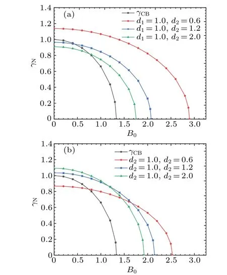
Fig. 8. The normalized linear growth rate γN versus the magnetic field intensity B0 for fixed dimensionless thickness of the upper fluid d1 (a) and for fixed dimensionless thickness of the lower fluid d2 (b). The relevant parameters are k=2,ρ1=8,ρ2=1,U1=1,U2=−1,µ0=1,LB=0.

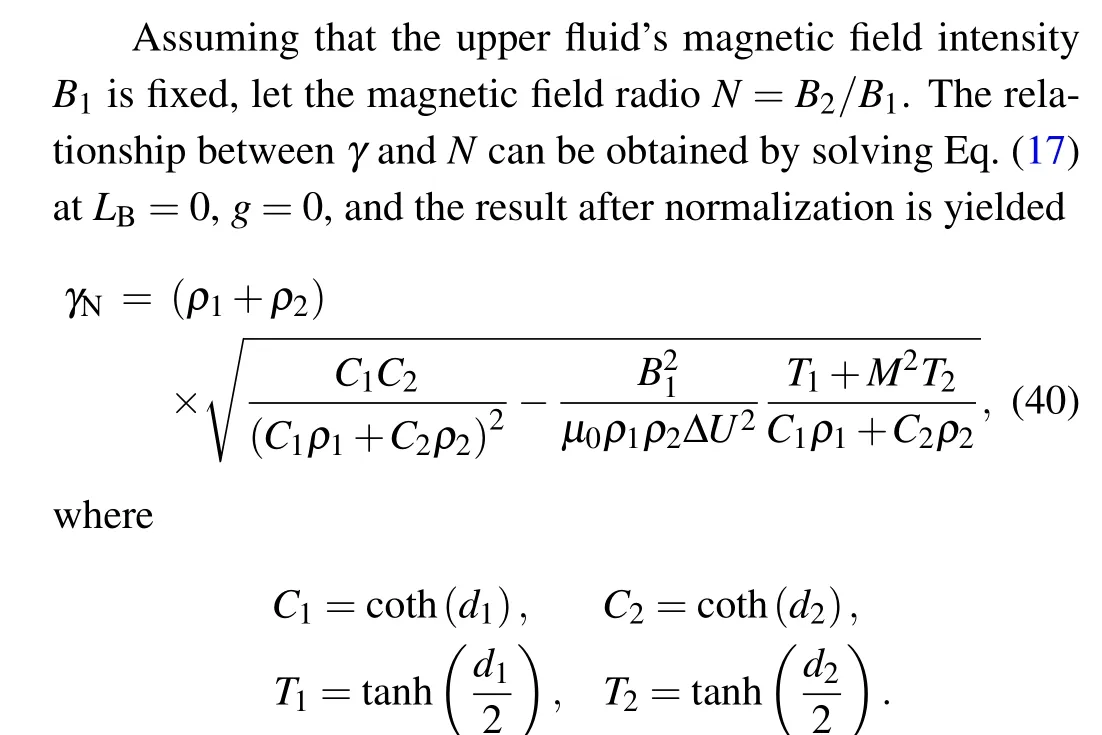
LetR=ρ2/ρ1be the density ratio,figure 9 shows the relation amongγN,R,andN. As shown in Fig.9,γNdecreases withN,and the largerNis,the fasterγNdecreases. For fixedN,γNincreases withR. These conclusions hold for both the finite and infinite thickness cases.[13]

AtLB/=0, we derive an explicit analytic expression for the linear growth rateγof the KHI for finite-thickness fluids under the influence of a continuous magnetic field profile.Figure 10 shows the relationship between the normalized linear growth rateγNand the ratio of the magnetic fieldNwith different ratios of densityR. We find that in the case of continuous magnetic field profile, the ratioNof magnetic field intensity plays the same destabilizing effect on KHI,while the density ratio remains destabilizing. This is consistent with our conclusion in the presence of discontinuous magnetic fields.

Fig.9.The relations among the ratio of the magnetic field N,normalized linear growth rate γN,and density ratio R with k=8,ρ1=5,U1=1,U2=−1,B1=0.5,µ0=1,LB=0,d1=d2=4(The magnetic field profile is discontinuous).

Fig.10. The relations among the ratio of the magnetic field N,the normalized linear growth rate γN and density ratio R with k=8, ρ1 =5,U1 =1,U2 =−1, B1 =0.5, µ0 =1, LB =0.9, d1 =d2 =4 (The magnetic field profile is continuous).

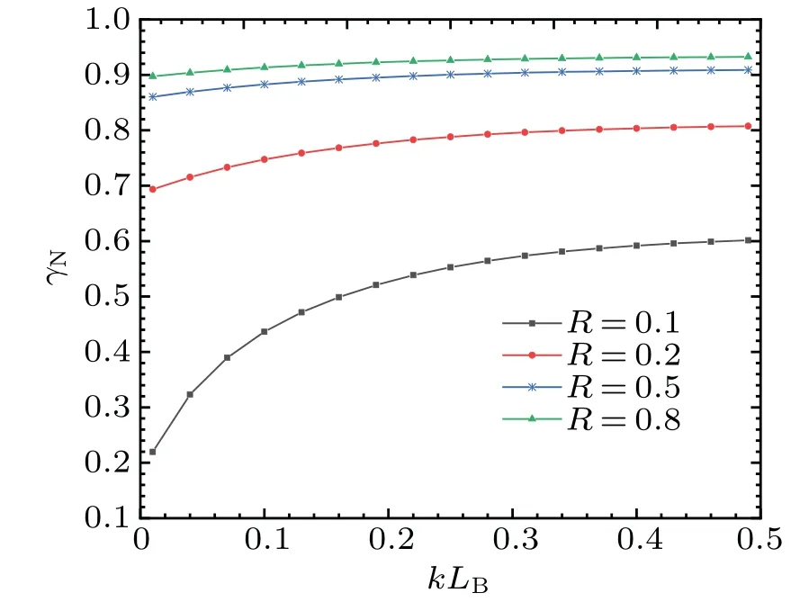
Fig. 11. The normalized linear growth rate versus dimensionless magnetic field gradient scale length kLB with fluid dimensionless thickness d1 =d2 =0.5 and for fixed R=0.1, 0.2, 0.5, 0.8. The other parameters are ρ1=4,U1=1,U2=−1,µ0=1,B1=3.5,B2=0.5,k=1.

Figure 11 shows the effect of the dimensionless gradient scale lengthkLBof the magnetic field on the normalized linear growth rate of the KHI for finite-thickness fluid. As shown in Fig. 11,γNincreases withkLB, and the growth rate ofγNis faster in the case of smallerkLB. This growth effect is less obvious in the case of larger density ratioR. At the same time,γNincreases withRfor fixedkLB. This conclusion is similar to the one drawn in the infinite plane.[13]When the values ofkLBis larger enough,γNcan be saturated.

Based on the practical application of experimental scheme of double-cone ignition described in the previous section,we will discuss the effect of the total thickness in combination with the external magnetic field on the linear growth of the KHI.

We still assume that the upper fluid’s magnetic field intensity is equal to the lower one(B1=B2=B0),then we obtain

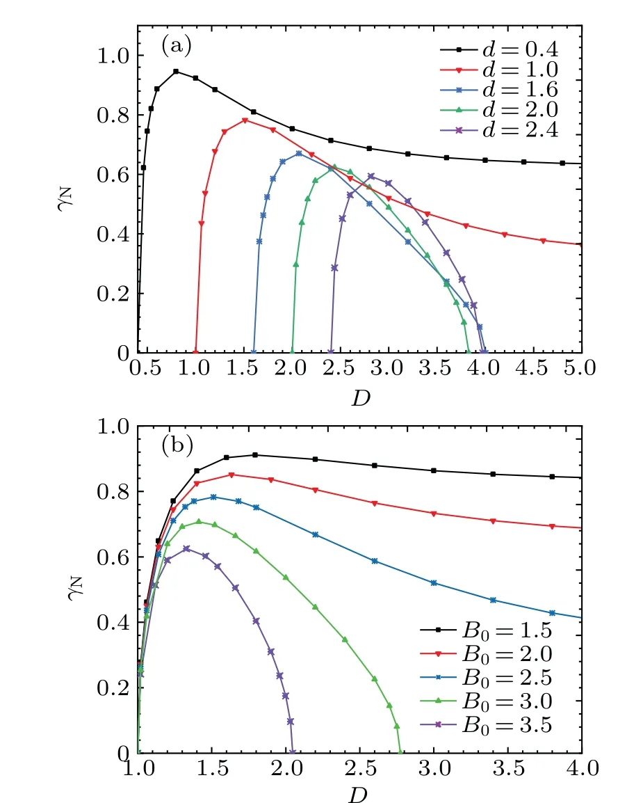
Fig.12. The relations among the dimensionless total thickness D, normalized linear growth rate γN, and the dimensionless initial given thickness d(a)with k=2,ρ1=4,ρ2=5,∆U =2,µ0=1,B0=2.5,d=0.4,1.0,1.6,2.0,2.4. The relations among D,γN,and the magnetic field intensity B0 (b)with k=2,ρ1=4,ρ2=5,∆U =2, µ0=1,d=1,B0=1.5,2.0,2.5,3.0,3.5.

We choose the case ofρ1<ρ2for discussion. Figure 12(a) displays that for fixed magnetic field intensity, the sensitivity of the normalized linear growth rate of KHI to the dimensionless total thickness varies for fluids with different initial dimensionless thicknesses. When the initial dimensionless thickness is small,γNincreases rapidly withDto a maximum value and then gradually decreases. However,when the initial dimensionless thickness is high,γNdecreases rapidly after reaching the maximum value and can even decrease to zero,which means KHI is completely suppressed. The larger the value of the initial dimensionless thicknessdis,the smaller the maximum value ofγNreaches. It is seen in Fig. 12(b),for fixedd, the variation curve ofγNwithDis similar to the curve of fixedB0in Fig.12(a). For fixedD,γdecreases withB0. When the magnetic field intensity is larger,the maximum value thatγNcan reach is smaller,andγNdecreases faster withD. These conclusions suggest that in addition to selecting the proper total thickness of coating in the specific experiments of double-cone ignition scheme,we can also make full use of the suppression effect of magnetic field on KHI in order to reduce the linear growth of KHI. If we consider the effects of thickness and magnetic field together, the inhibition may be more obvious.

4.3. Extended applications

Our theoretical model can also be applied to related experiments on the effect of magnetic field on the linear growth of KHI in laser driven plasmas. Sunet al.[19]have presented the experimental results of a KHI produced by intense laserdriven thin plastic foils with external magnetic field. The relevant parameters in the article arek ∼4πµm−1,ρ1∼ρ2∼1019cm−3,U1∼138.2 km/s,U2∼0,B0∼1424 Gs(1 Gs=10−4T)and the thickness of the plastic foil is 10µm.According to the conclusions we drawn from the previous sections, if we take the thickness of the plastic foil into account,we may get an in-depth physical understanding of the KHI of fluid with finite thickness.

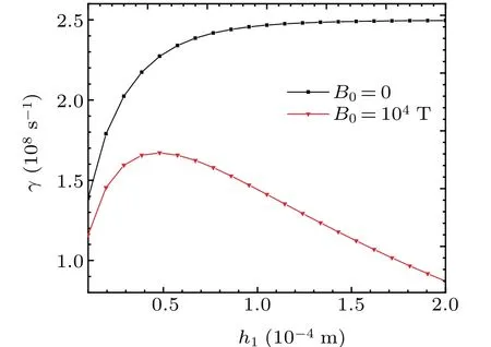
Fig.13. The effect of the fluid thickness with and without the external magnetic fields for parameters closely related to the ICF implosions. The vacuum permeabilityµ0 ≈1.26×10−6 H/m. h2=6×10−4 m.

Figure 13 illustrates the effect of the fluid thickness on the linear growth rate using parameters closely related to the maximum compression of the ICF implosions. The parameters are:[20]k= 104m−1,ρ1= 1.3×105kg/m−3,ρ2=1.2×105kg/m−3,U1=4×105m/s,U2=3.5×105m/s.In ICF implosion experiments, the growth of KHI may also occurs due to the change of fluid thickness, which can be inhibited by the presence of an external magnetic field. Our theoretical model may be applied to related experiments in ICF in the future.

5. Conclusion

In summary, the magnetic field effect still has a strong suppression of KHI when the fluids have a finite thickness,but a stronger magnetic field is required to achieve the same suppression compared to the case of infinite planes. When the effect of the magnetic fields is neglected,the analysis yields that reducing the fluid thickness on the denser side or increasing the fluid thickness on the less dense side can both suppress the linear growth of KHI. Considering the effect of the magnetic field,the thickness of fluids and the magnetic fields acting together on the linear growth of KHI.It is found that increasing the thickness on the less dense side of the fluid can still suppress the linear growth of KHI, while reducing the thickness on the denser side of the fluid can only achieve the same effect when the external magnetic field intensity is small.If the magnetic fields are continuously distributed, we find that the normalized linear growth rateγNincreases with the magnetic field gradient scale lengthkLBwhen the magnetic field intensity is strong. When considering the effect of the dimensionless total thickness of fluidsD,the normalized linear growth rateγNof KHI increases rapidly withDand reaches the maximum value,then decreases withDor remains constant. During the decrease ofγN, the larger the value of the initial dimensionless thicknessdis,the more slowlyγNdecreases withD. With the effect of the magnetic field, the linear growth of KHI always decreases with the increasing of the total thickness after reaching a maximum value. The stronger the magnetic field intensity is, the more obvious the growth rate decreases with the total thickness. If we consider the effect of the total thickness and magnetic field together under specific experimental conditions,a more obvious suppression result of KHI may be obtained. These conclusions may provide a theoretical reference to the experimental results of a KHI produced by intense laser-driven thin plastic foils with external magnetic field[19]and to the suppression of KHI in the thin film layer(coating)in Zhang’s[18]double-cone ignition scheme. Finally,we compare the analytic linear growth rates with numerical results,and they agree well with each other.

Acknowledgements

Project supported by the Strategic Priority Research Program of the Chinese Academy of Sciences (Grant Nos. XDA25051000 and XDA25010100) and the Fundamental Research Funds for the Central Universities (Grant No.2022YQLX01).