Variational quantum eigensolvers by variance minimization

Dan-Bo Zhang(张旦波) Bin-Lin Chen(陈彬琳) Zhan-Hao Yuan(原展豪) and Tao Yin(殷涛)

1Guangdong–Hong Kong Joint Laboratory of Quantum Matter,Frontier Research Institute for Physics,

South China Normal University,Guangzhou 510006,China

2Guangdong Provincial Key Laboratory of Quantum Engineering and Quantum Materials,School of Physics and Telecommunication Engineering,South China Normal University,Guangzhou 510006,China

3Guangzhou Educational Infrastructure and Equipment Center,Guangzhou 510006,China

4Yuntao Quantum Technologies,Shenzhen 518000,China

Keywords: quantum computing,quantum algorithm,quantum chemistry

1. Introduction

The variational principle is instrumental for understanding physical theories and also becomes a powerful tool for solving computational physics problems. In recent years,the power of quantum computing of near-term noisy quantum processors is expected to be exploited with variational methods,[1–24]which refers to hybrid quantum-classical algorithms for optimization. A representative example is variational quantum eigensolver (VQE),[1,3,7,15,19,22]which receives special interests due to its fundamental roles in quantum chemistry,[1,3,7,22,25]quantum many-body systems,[13,19]and many other applications.[9,26,27]

Interestingly,though called eigensolver,the original VQE is designed to solve the ground state for a Hamiltonian,since it uses the energy as a cost function to minimize,which promises to give an upper bound for the ground state energy. For being an eigensolver, many variants of VQE have been developed to solve excited states,which can be understood as minimizing energy in a subspace, constrained by symmetries,[28]enforced by orthogonality,[29]obtained by eliminating the space of lower energy states,[16]or using quantum subspace expansion.[5]As excited states are responsible for physical processes such as chemical reactions, advances in VQE for calculating excited states are arguably important.

While those variants of VQE can be successful to some extent, an alternative approach is to directly access whether a state is an eigenstate and use this criterion as a cost function to optimize. A simple answer for this is to use zero energy variance to judge an eigenstate, since an eigenstate should have zero energy variance. Variational methods based on the zero-energy variance principle that run on classical computers,[30–36]in fact,can be originated in the early age of quantum mechanics for solving the Helium atom.[30]Remarkably,zero variance puts a very strong constraint on the wavefunction structure, and it can be powerful for solving quantum many-body problems when a well-approximated wavefunction is required.[35]The zero-variance principle has been applied experimentally to self verify if a quantum simulator can prepare a ground state for a Hamiltonian.[13]It is, however,awaiting for exploiting the power of quantum computing to develop a variational quantum eigensolver that is based on minimizing energy variance,which can solve ground state and excited states on the same footing.

In this paper, we develop a variational quantum eigensolver based on minimizing energy variance,and we call it the variance-VQE. For solving excited states of a Hamiltonian,we give two approaches, which represent eigenstates in different ways. One uses a single wavefunction ansatz, where different parameters correspond to different eigenstates. The other uses a set of orthogonal wavefunction ansatzs,and incorporates energy variances into one cost function for optimization. We numerically solve the energy potential surface for molecules, which is a fundamental quantum chemistry problem, and demonstrate the properties of variance VQE as well as explore its potential advantages. We also show that optimizing a combination of energy and variance may be more efficient in finding a set of eigenstates with lowest energies,compared with one that optimizes energy or variance alone.Moreover,we investigate stochastic gradient descent for optimizing the variance-VQE with Hamiltonian sampling, which can be useful for optimization with fewer quantum resources.Our work demonstrates that VQE by minimizing energy variance can be useful for calculating excited states and also for working out an avenue to reach efficient optimization.

The paper is organized as follows. We first propose variance VQE in Section 2,and then apply it to solve excited states for quantum chemistry problems in Section 3.In Section 4,we investigate the stochastic gradient for optimizing the variance-VQE.Finally,we give a summary in Section 5.

2. Variance VQE

In this section, we first review the traditional approach of variational quantum eigensolver that minimizes the energy.Then, we formulate a new type of VQE that minimizes the energy variance and then discusses its optimization.

2.1. VQE by energy minimization

We consider a HamiltonianHas a summation of local terms,H= ∑Ni=1ciLi, where a local HamiltonianLican be written as a tensor product of a few Pauli matrices. We denotec=(c1,c2,...,cN)TandL=(L1,L2,...,LN)T. Thus we can writeH=cTL.

The variational quantum eigensolver works as follows.One uses an ansatz|ψ(β)〉=U(β)|R〉to represent a candidate ground state.Here|R〉usually is taken as an approximation for the ground state ofH,e.g.,Hartree–Fock state for the quantum chemistry problem.U(β)is a unitary operator parameterized withβ. The task then is to optimizeβfor some cost function.The traditional way is to minimize the energy defined as

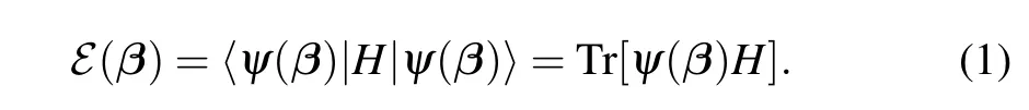
Here, we have denotedψ(β)=|ψ(β)〉〈ψ(β)|. By designing, VQE based on minimizing energy is suitable for finding ground state of a Hamiltonian.

The optimization is completed with a hybrid quantumclassical algorithm. The quantum processor preparesψ(β)and performs measurements to evaluateℰ(β), which can be reduced intoℰ(β) =cTℒ(β), whereℒ(β) = Tr(ψ(β)L).Here, quantum average of each component ofLcorresponds to a joint measurement on multiple qubits. The classical computer updates parametersβaccording to received data from the quantum processor, which forms a hybrid quantumclassical optimization loop.

2.2. VQE by variance minimization

As the name indicates, variational quantum eigensolver should aim at solving eigenstates. However, VQE, based on minimizing energy,is prone to find only an eigenstate with the lowest energy, named as the ground state. Other VQEs have been developed for solving excited states. Essentially, those VQEs are realized by minimizing energy in a subspace,which is enforced with symmetry, or by eliminating space of lower energy states with an orthogonality condition.

Can variational quantum eigensolver directly solve excited states? An answer for this is to design a cost function that can assign the same cost to all eigenstates and higher cost for other states. A natural choice is energy variance, which is zero only for eigenstates and positive for others. By minimizing energy variance, one can then find the eigenstates of a Hamiltonian. We call these two methods the minimized energy variance-VQE and energy-VQE,respectively.

Let us formulate variance-VQE. The energy variance of HamiltonianHwith a wavefunctionψ(β)can be written as

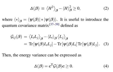
The non-negative energy variance consists ofG(β),which is a semi-positive matrix. Note that each element ofG(β)can be obtained on a quantum computer. Then, the energy variance can be evaluated based on the quantum covariance matrix.

As a variational method,one key ingredient for variance-VQE is whether the wavefunciton ansatz has enough expressive power to parameterize the eigenstates. Unlike energy-VQE which looks for a ground state,the chance that an ansatz can parameterize some eigenstates can be greater as there are 2Meigenstates for a quantum system ofMqubits, although it is in general hard for an ansatz to parameterize all eigenstates. Notably, with an intermediate-size variational quantum circuit,it is expected that lower-lying eigenstates may be parameterized, as those states typically will be characterized with smaller entanglement entropy.[40]This can be useful as most applications are interested in lower-lying eigenstates. In addition,the variance-VQE has the self-verifying property that it can verify whether it indeed obtains an eigenstate by checking if the energy variance is zero.

Another important aspect is optimization, namely minimizing the energy variance, which can be carried with gradient free or gradient descents. The gradient descent method requires to calculate the gradient of energy variance,which is

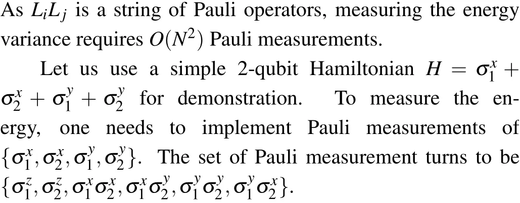
SinceG(β) should be evaluated withO(N2) elements,calculating energy variance costsO(N2),which is larger than a cost ofO(N) for calculating energy (see Appendix for details as well as a demonstrative comparison using a 2-qubit Hamiltonian).As a result,direct gradient descent for variance-VQE can be more resource-costing than energy-VQE. Nevertheless, we can use Hamiltonian sampling to reduce this cost,[42]which estimates the energy variance and its gradient by sampling only a portion of the quantum covariance matrix. In Section 4, we will give a stochastic gradient descent algorithm for optimizing variance-VQE by Hamiltonian sampling,[42]which can be efficient under a minimal sampling rate and thus can reduce the overload significantly. Moreover,one may reduce the overload of evaluating the energy variance by using some smarter strategies that can simultaneously access a set of quantum covariance matrix elements,[43,44]or use the quantum power method introduced in Ref.[45].

3. The variance-VQE for excited states

As all eigenstates always have zero variance, optimizing the variance-VQE by minimizing energy variance may lead to any eigenstate. Thus, the variance-VQE can be used for obtaining excited states. In this section,we propose different approaches for solving excited states of molecule Hamiltonians with the variance VQE. We first show that the cost function variance-VQE can have many global minimums of zero variance,corresponding to different excited states. However,this approach can be inefficient if a specified eigenstate is required.To overcome this,we propose the variance-VQE that solves a set of excited states jointly, using a set of orthogonal wavefunction ansatzs. We further demonstrate that optimization of a linear combination of energy and variance can be more efficient than optimizing energy or variance alone.

For demonstration, we use the hydrogen moleculeH2as an example. We would consider a more complicated system,H4, in Section 4. All Hamiltonians are calculated withOpenFermion,[46]and the numeral simulation for the variance VQE is conducted with the HiQ simulator framework.[47]Under STO-3G basis, we use four qubits to describe the Hamiltonian ofH2. A UCC ansatz is taken with trotter stepk=1(see Appendix B),and there are 9 parameters(6 for single excitations and 3 for double excitations). The reference state is chosen as|0011〉,or others in the subspace of two electrons.

Though demonstrated with UCC ansatz for quantum chemistry problems, it should be stressed that the framework of variance-VQE can be applied for solving general quantum systems with proper chosen ansatz. The choosing of ansatz is often domain specific and can be important for efficiently applying VQE.For instance, to solve quantum lattice models one may adopt the Hamiltonian variational ansatz.[48]

3.1. Single ansatz with multiple global minimums

For the variance VQE,the criterion for being eigenstates is that energy variance∆(β)=0. If a wavefunction ansatz can represent all eigenstates,then we can expect that there are many solutions ofβcorresponding to∆(β)=0. In practice,as high energy eigenstates usually have higher complexity,an ansatz may only capture some eigenstates.In the optimization,one can select those minimums that are close to zero. This is indeed one advantage of the variance-VQE: one can verify if an eigenstate is obtained by checking whether the variance is zero.[13]A direct way to calculate excited states with the variance VQE is as follows. First, chose an ansatz|ψ(β)〉that can express considered excited states. For quantum chemistry,we can use some modified UCC ansatzs with enough singleparticle and double-particle excitations (see Appendix A).Second, minimizing∆(β) with random choice of initial parametersβ0∈[0,2π]K. Third,select minimums of∆(β)that are close to zero. Lastly, with optimized parameters, we can calculate their corresponding energies.

Fig. 1. Distribution of global minimums in the parameter space β,where the high dimension β is visualized on a plane by dimensional reduction,using multi-dimensional scaling method. E0,E1,E2,and E3 correspond to energy levels in ascending order.

As for demonstration, we calculate the spectrum ofH2.With uniformly sampled initialβ,we optimize the energy variance with default optimizer inScipy. All obtained minimums are almost zero (less than 10−8), and their corresponding energies are eigen-energies successfully. However, we find the chance to be a given eigenstate varies,e.g.,solutions to ground states are far less than excited states. To illustrate this, we visualize the distribution of solutions in the parameter space,as seen in Fig.1, by projecting the 9-dimensional parameters onto a plane,using a multidimensional scaling method that can preserve well information of distance. Note that we use a distance metricd(β,β′)=∑icos(θi −θ′i) asθis an angle such thatθ1=θ2mod 2π. This indicates that the ground state is relatively hard to find in this method. It is also observed that multiple points of parameters may correspond to excited states with the same energy. For non-degenerate eigenstates, corresponding toE0,E2,E3respectively, it can be explained that differentU(β)can transform|R〉to the same target state. As excited states forE1are three-fold degenerate(will be revealed later),there are many solutions ofU(β)that transforms|R〉to this subspace. We remark that the above phenomena hold for other reference states,e.g.,|0101〉and|0110〉.

3.2. A set of orthogonal ansatzs

While variance-VQE can be optimized to obtain all eigenstates for a single ansatz with different optimized parameters,it may be hard to get the ground state or other specified states as it requires choosing a proper initial parameter. Here we develop another method,using a set of orthogonal ansatz wavefunctions.

The orthogonality of ansatzs for different eigenstates can be easily enforced by using|ψn(β)〉=U(β)|Rn〉, where{|Rn〉}are orthogonal to each other. Note that all ansatz uses the sameU(β)and the orthogonality of{|ψn(β)〉}only holds under the sameβ. To optimizeβ,we use a cost function that is equal-weighting summation of all energy variances, which can be written as

where∆n(β)is the energy variance ofHfor the state|ψn(β)〉,andwn= 1/k. The formula is similar to that of subspacesearch VQE, which requires a specified weighting{wn}that enforces an ordering of eigenstates. We note that Eq. (7) has been used in Ref.[35]to calculate all eigenstates of quantum many-body systems with unitary matrix product state ansatz.

While other methods usually calculate excited states one by one, this method incorporates all into a single cost function to optimize. In spirit, it can be viewed as a multi-task learning.[49]As those tasks are closely related, solving them in a package may benefit each other.

Solving excited states then can be carried out by optimizingCvar(β)with gradient descent,

Other gradient-free methods are also applicable. We present the numeral results forH2. Reference states are computational basis on a subspace of two occupied electrons, which has 6 states. As the UCC ansatz is particle-conserving, the wavefunction ansatz is in the subspace of 2 particles. The energy potential curve fits perfectly to that by exact diagonalization,as seen in Fig. 2. It is interesting to note that there are only four energy levels,while the subspace is 6-dimensional. This can be explained that the first excited state is three-fold degenerate.

Fig. 2. The spectrum of H2 with different bond lengths. Blue dash lines are results from exact diagonalization in the whole Hilbert space.Red markers are obtained from the variance-VQE in a subspace of two electrons that H2 is electronic neutral.

Moreover, evaluation of the cost function Eq. (7) can be more efficient with ancillary qubits, which is given in Appendix C. This is useful when lots of eigenstates are needed,where a direct summation can be impractical. For instance,there is an exponentially large number of terms when all eigenstates are needed.

It is interesting to compare the result of the variance-VQE with orthogonal ansatz to that of subspace-search VQE.[29]The subspace-search VQE focuses on a subspace of eigenstates function and optimizes a number ofklow-energy eigenstates simultaneously. The cost function is a weighted combination of all energies,

where|ψn(β)〉=U(β)|n〉. The weightings satisfyw0>w1>w2>···>wk−1, such that energies at optimizedβ∗will satisfyℰ0(β∗)≤ℰ1(β∗)≤···≤ℰk−1(β∗) (see the proof in Ref.[29]). It is noted that the weightings can be learned,as in Ref. [20], which self adjusts the weightings when variational preparing Gibbs state for a quantum system.

One requirement for the subspace-search VQE is that the order of eigenstates needs to be given. It is possible that the optimization may go a long way to make all eigenstates rest in a given order, as revealed in Fig. 3. This can increase the complexity of the optimization. To illuminate this, we compare the evolution of energies in the optimization process for both subspace-search VQE and variance-VQE. The ordering of eigenstates in the subspace-search VQE is fixed by reference states|0011〉,|0101〉,|1001〉,|0110〉,|1010〉,|1100〉,which give to ascending order of energies after optimization.As seen in Fig.3,initialized with the same parameters and thus the same energies, evolutions of energies for subspace-VQE will have complicated trajectories toward convergence.In contrast, all orthogonal ansatz wavefunctions flow directly to the nearest eigenstates in the variance-VQE.We also check other ordering of eigenstates for the subspace-search VQE,and find the same result.

Fig.3. Evolution of energy levels in the process of optimization. Two methods are compared: the subspace-search VQE and the variance-VQE.The bond length for H2 is λ =1.

3.3. Minimizing a combination of energy and variance

For the orthogonal ansatz, if we only choose a subset of the Hilbert space or subspace with a fixed number, then the variance-VQE can not promise that the solutions are lowest energy states. Just as the previous approach uses one ansatz,the final result depends on the initial parameter and the optimization process. On the other hand,for a cost function with an equal-weighting energies for orthogonal ansatz, it can get the lowest total energy, but can not promise each optimized state to be an eigenstate. While subspace-search VQE can solve this problem, the optimization can not be efficient by assigning an order for ansatzs as eigenstates.Here,we demonstrate that a simple combination of energies and energy variances can make the best of both to find low energy excited states.[33]The cost function as a combination of energies and energy variances can be written as

In this regard, the optimization includes gradient information of both energy and energy variance,andηvplays a role in adjusting the step size between them. In Fig. 4, we show the result of mixed VQE with differentηv,and it can be seen that nonzeroηvis critical to get the right eigenstates,and increasingηvcan raise the efficiency for optimization. Moreover, if only energy variance is used in the cost function,the solution may not be the lowest energy eigenstates. Thus, the result demonstrates that a combination of energy and energy variance can be useful and efficient for VQE to solve low-energy excited states.

Fig. 4. Optimization processes for mixed cost function with different mixing factor ηv of energy variances. Three orthogonal ansatzs are used. The bond length for H2 is λ =0.8.

4. Hamiltonian sampling

So far,we have demonstrated that the variance-VQE can efficiently solve excited states for a Hamiltonian. However,the overload of calculating variance and its gradient descent is massive since it scales with the number of Hamiltonian terms asO(N2). In this section, we propose stochastic gradient descent for the variance-VQE by Hamiltonian sampling, which can significantly reduce the overload.

The Hamiltonian sampling randomly choose some components ofc(setci=0 ifciis not chosen),which is denoted as ˜c. Then,the estimated energy variance is A prefactor|c|2/˜c2is added to account for the fact that coefficients for different terms of a Hamiltonian vary largely, so there should be a term for normalization. Whenever ˜ci=0,elementsG(β)i jdo not need to be evaluated. For a sampling rates(defined as a ratio thatciis sampled),the number of elements inG(β)ijrequired to be calculated can be reduced to a factors2.

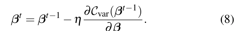
With a Hamiltonian sampling, the gradient can be estimated as∂˜∆(β)/∂β, which shall have a distribution due to sampling. With this gradient, a stochastic gradient descent algorithm can be applied for optimizing the variance-VQE,which updates parameters as

We apply the stochastic gradient descent for solving eigenstates ofH2andH4with the variance-VQE. The moleculeH4is investigated in a trapezoidal structure. Under sto-6g basis,we use a Hamiltonian of 6 qubits to describeH4.The UCC ansatz is chosen ask=1 with 21 parameters,including 15 for single-particle excitations and 6 for double-particle excitations(we only consider double-particle excitations from occupied orbitals to empty orbitals). Note that there are more than one hundred terms for the Hamiltonian,which means that Hamiltonian sampling is badly demanded to evaluate the variance.

Numeral simulation results are displayed in Fig. 5 for solving two eigenstates with orthogonal ansatzs. ForH2, it shows that Hamiltonian sampling with a small sampling rates=0.1,0.2 can have comparable convergent behavior with the case without sampling. However, the variance ceases to converge at small values, due to the fluctuation of energy for a subsystem even when the whole system has zero energy variance. To solve this issue, we can turn to no sampling (sampling rates=1) in the later stage of optimization. ForH4,similar phenomena can be observed. It is noted that only one ansatz reaches the true eigenstate, while the other fail (a local minimum or the ansatz lacks the capacity to express this eigenstate), which can be seen from the nonzero energy variance.This again verifies that the variance-VQE can self-verify whether an eigenstate is obtained.

Fig.5. Optimization of the variance-VQE for H2 (upper row)and H4 (down row)with different Hamiltonian sampling rates s. Sampling rates can be adjustable in an optimization process,for instance,s=0.1 and 1 means that s changes from 0.1 to 1 in the later stage of optimization.The learning rate is 0.05 for all cases.

We can explain why Hamiltonian sampling fails to work around the optimized point of parameters,where gradients by Hamiltonian sampling can give meaningless direction for optimization. This is because energy variance is not additive: ifH=HA+HBand the wavefunction is|ψ〉, then the variance ofHis not a summation of the variances ofHAandHB. For example,if|ψ〉is an eigenstate ofH,|ψ〉will not be an eigenstate ofHAorHB,if A and B are entangled.As a result,even at the optimized parameter of zero variance,gradients by Hamiltonian sampling can be finite. Such a property is in sharp contrast to the case of machine learning.Machine learning usually uses a set of independent and identically distributed samples,and the cost function is a summation of independent contributions from all samples. Thus,gradients can be estimated with a batch of samples, giving stochastic gradient descents with well convergence behavior.[50]

From the above discussion, a practical strategy is to use Hamiltonian sampling with a small sampling rate to optimize the variance to a small value, then turn to a large sampling rate or no sampling. Also,one may then use energy-VQE.We note that stochastic gradient descent with few shots of measurements can further reduce the overload,[42,51]which leaves for further investigation.

5. Summary

In summary,we have proposed the variance-VQE that optimizes the energy variance to obtain eigenstates for a Hamiltonian. Compared with the VQE that minimizes the energy which is prone to find ground state, the variance-VQE naturally is suitable for solving and self-verifying arbitrary eigenstates. We have adopted different strategies to solve excited states with the variance-VQE, using moleculesH2andH4as examples. Remarkably, it has been shown that optimizing a set of orthogonal ansatzs with the same parameterized circuit can be very efficient for calculating a set of eigenstates. Also,we have demonstrated that minimizing a linear combination of energy and variance can outperform the case of optimizing either energy or variance alone. Moreover, we have proposed stochastic gradient descent for minimizing the variance by Hamiltonian sampling, using only a few terms of the Hamiltonian to estimate the variance and its gradient. It has been shown that the variance can decrease quickly under a small sampling rate. While numeral simulations suggested that the variance fails to converge, Hamiltonian sampling can be useful in the early stage to locate the zone of optimized parameters. Our work has demonstrated that the variance-VQE can be useful and practical for variational solving excited states in a quantum system on a quantum computer.

Appendix A: Comparison between measurements of energy and variance

For a HamiltonianH= ∑Ni=1ciLi, whereLiis a Pauli string, it is known that measurement of the energy with regard to a wavefunction|ψ〉can be carried out by measuring everyLiseparately and then making a linear combination of results ofNPauli measurements,namely,The capacity of decomposing the energy measurement to simple Pauli measurements is key for implementing variational quantum eigensolver.

The situation is similar for measuring the energy variance on the quantum computer. One can make a decomposition for the first term in Eq.(2),

Appendix B:UCC ansatz

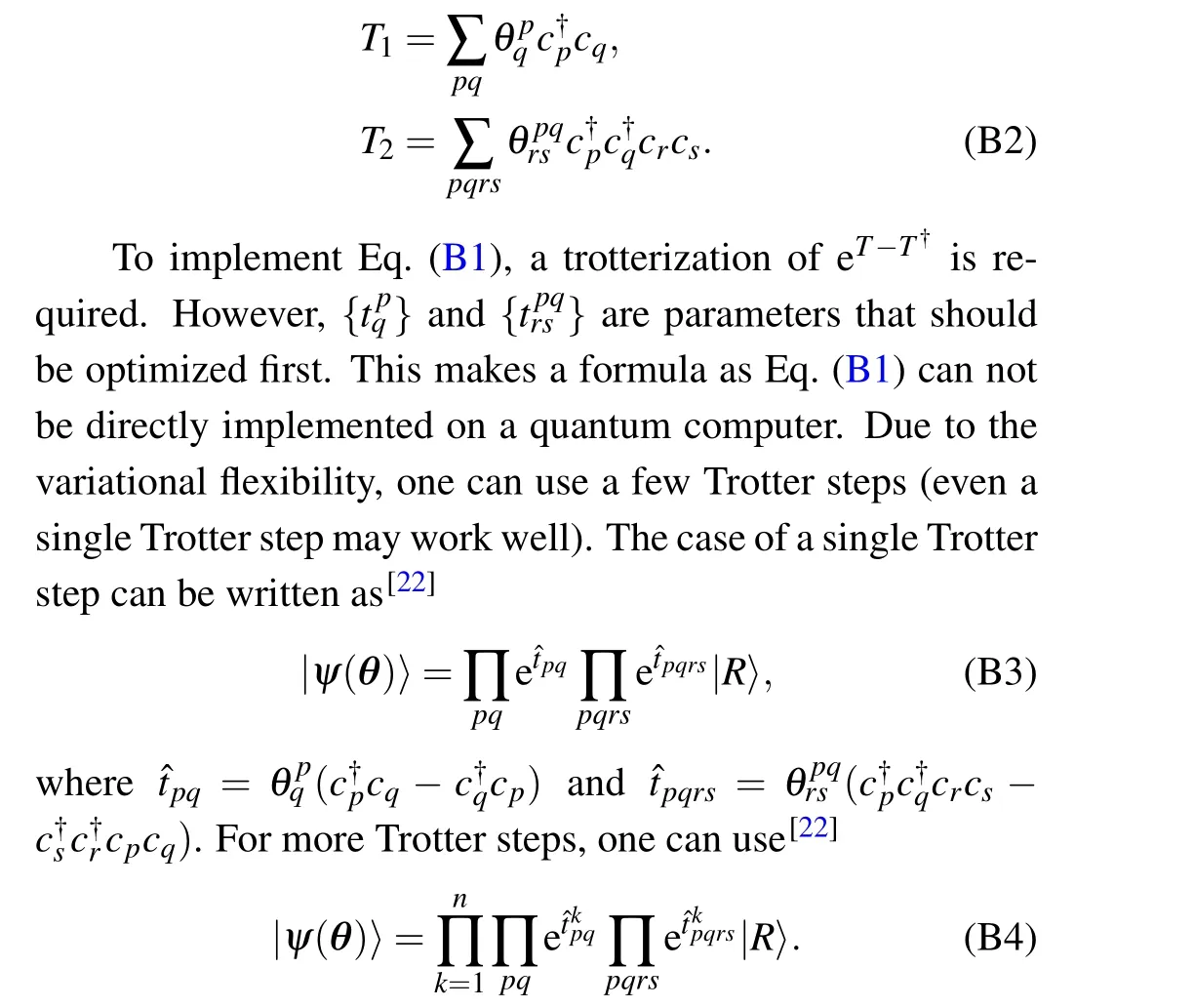
The UCC ansatz is widely used in the field of quantum chemistry,as it can represent a parameterized wavefunction of electronic structure of a molecule efficiently. The parameterized wavefunction can be written as Here,T=T1+T2usually includes single-particle excitationsT1and double-particle excitationsT2. We adopt a notation that does not distinguish occupied and empty states in the reference state|R〉(which typically is a Hartree–Fock state). ThenT1andT2can be expressed as

Appendix C:Efficient evaluation of cost function

While the goal is to solve a number ofkexcited states,evaluation of the cost function (the total energy variance) is time-consuming for largek, since it should calculate energy variance one by one. For instance, for a system ofMqubits,the total number of eigenstates is 2M. Here, we discuss how to efficiently evaluateCvar(β),similar to Ref.[35]. Let us first considerk=2M. Using then it can be verified that

To evaluate the second part of Eq. (7), the summation in Eq. (C4) should be replaced byk −1. The total number of qubits isM+M+W=2M+W.

Acknowledgements

This work was supported by the National Natural Science Foundation of China (Grant No. 12005065) and the Guangdong Basic and Applied Basic Research Fund (Grant No.2021A1515010317).