Estimating Ground Snow Load Based on Ground Snow Depth and Climatological Elements for Snow Hazard Assessment in Northeastern China

Huamei Mo · Guolong Zhang · Qingwen Zhang ·H. P. Hong · Feng Fan

Abstract Extreme snow loads can collapse roofs. This load is calculated based on the ground snow load (that is,the snow water equivalent on the ground). However, snow water equivalent (SWE) measurements are unavailable for most sites, while the ground snow depth is frequently measured and recorded. A new simple practical algorithm was proposed in this study to evaluate the SWE by utilizing ground snow depth, precipitation data, wind speed, and air temperature. For the evaluation, the precipitation was classif ied as snowfall or rainfall according to the air temperature,the snowfall or rainfall was then corrected for measurement error that is mainly caused by wind-induced undercatch, and the eff ect of snow water loss was considered. The developed algorithm was applied and validated using data from 57 meteorological stations located in the northeastern region of China. The annual maximum SWE obtained based on the proposed algorithm was compared with that obtained from the actual SWE measurements. The return period values of the annual maximum ground snow load were estimated and compared to those obtained according to the procedure suggested by the Chinese structural design code. The comparison indicated that the use of the proposed algorithm leads to a good estimated SWE or ground snow load. Its use allowed the estimation of the ground snow load for sites without SWE measurement and facilitated snow hazard mapping.

Keywords Ground snow depth · Ground snow load ·Northeastern China · Precipitation data · Snow hazard mapping · Snow water equivalent

1 Introduction

Roof snow load for codif ied structural design is based on the basic ground snow load and a ground-to-roof factor. The basic ground snow load in the Chinese load code (MOHURD 2012) is assigned based on theT-year return period value of the annual maximum ground snow load, whereTis equal to 50 years. The basic ground snow load could be estimated based on the historical records of the measured ground snow load, or snow water equivalent (SWE). However, this kind of historical record is available for only a few meteorological stations, while ground snow depth records are more widely available for many meteorological stations.This is because the resources required to measure the SWE are much greater than those needed to measure snow depths(Sturm et al. 2010). Consequently, it is valuable to infer or estimate ground snow load from ground snow depth. This could augment the SWE database and result in a better spatial representation of ground snow load, which can be used to estimate the nominal ground snow load in the context of structural design codes (Hong and Ye 2014; Mo et al. 2016).

There have been several eff orts to estimate the ground snow load from the ground snow depth, including Fridley et al. ( 1994), Jonas et al. ( 2009), McCreight and Small( 2014), Bruland et al. ( 2015), and Hill et al. ( 2019), among others. For the estimation, the snow depth and snow load (or SWE) are considered to be directly related by the snowpack bulk density. The snowpack bulk density is a function of snow depth, air temperature, air humidity, snow accumulation history, and other climatological variables (Ellingwood and Redf ield 1983; Sanpaolesi 1998; Sturm et al. 2010).Consequently, it could be feasible to estimate ground snow loads using these relevant climatological variables and the ground snow depth.

For example, Fridley et al. ( 1994) considered the measurements from a so-called f irst-order station (stations at which the SWE is recorded) in the United States and modeled the daily SWE using snow depth and daily average temperature. The proposed model was used to estimate ground snow loads for sites associated with a second-order station,where measurement of the SWE is unavailable. Jonas et al.( 2009) developed a snow density model for sites in Switzerland using season, snow depth, site altitude, and site location as input variables. Their analysis represented the relationship between snow density and snow depth by a linear function with model coeffi cients, which depend on the season,altitude, and site. They indicated that the model variability was of the same order of magnitude as that obtained based on measured snow density at a site. The model developed in Sturm et al. ( 2010) includes the eff ects of snow depth,snow aging–that is, day of the year (DOY)–and region.The model parameters were estimated by using a large number of snow measurement records from the United States,Canada, and Switzerland. The developed model allows the SWE to be estimated from the observed snow depth. Hill et al. ( 2019) regressed the SWE against snow depth, DOY,winter precipitation, and temperature using the measured SWE and the corresponding snow depth from the western United States and British Columbia. In their model, the snow season was separated into the accumulation phase and the ablation phase. An equation was given to evaluate the snow density for each phase. In both phases, the SWE was modeled as a power function of snow depth, DOY, winter precipitation, and temperature. They indicated that their model outperforms some other available models in the literature.A more extensive review on the estimation of the SWE from snow depth is available in Bean et al. ( 2021), who also proposed an algorithm based on a random forest model and found that it outperforms all existing methods for the U.S. dataset they considered. The random forest model is based on the machine learning technique, which is actually a regression approach (Breiman 2001) and this implies that it is not physically-based.

To develop a physically-based algorithm for evaluating the SWE by using ground snow depth measurements,none of the outlined studies directly used precipitation data as the main input variable to estimate the SWE, although precipitation is an important indicator of the SWE. This may be partly due to the diffi culties in collecting the gauge precipitation measurements, determining the fraction of precipitation that falls as snow, and estimating the water loss due to melting and/or evaporation. If the winter precipitation in cold regions represents the snowfall, especially during the accumulation period, the precipitation increment should be equal to the SWE increment. In such a case, if the water loss due to melting and/or evaporation could be estimated,the precipitation data could be directly used to estimate the SWE.

In this study, a new practical algorithm to estimate the SWE is proposed. The algorithm is based on frequently collected records of climatological elements such as precipitation, wind speed, temperature, and ground snow depth. The algorithm uses adjusted precipitation data and an estimation of snow water loss to calculate the SWE. The developed algorithm is applied to estimate the SWE for 57 meteorological stations located in the northeastern region of China.The annual maximum SWE obtained by using the proposed algorithm was compared with that obtained from the actual SWE measurements. Moreover, the application of the proposed algorithm to estimate the SWE for sites without actual SWE measurements was carried out. The obtained annual maximum SWE was used to map the snow hazard for the considered region. The climatological data, as well as the proposed algorithm, are described in the following sections.This is followed by the validation and application of the algorithm in estimating the SWE and mapping the snow hazard.

2 Climatological Data and Data Processing

The location of 99 meteorological stations for the considered northeastern region of China, where the required climatological data are available, is shown in Fig. 1 a. These stations provided a good spatial coverage for the region.The relevant climatological data for this study–including(accumulated ground) snow depth, (accumulated ground)SWE, precipitation, wind, and temperature–from 1971 to 2018 were acquired from the China Meteorological Administration (CMA).1http:// data. cma. cnA review of the data indicated that SWE data are available for the 57 meteorological stations shown in Fig. 1 b, while the other variables are available for all 99 stations. The considered region is one of the main regions in China associated with heavy snowfall. The mean winter temperature (averaged for December, January, and February) for some areas of this region is as low as −27 °C (Fig. 1 c), and the annual mean winter total precipitation could reach 41.5 mm for some locations (Fig. 1 d). For such a region, estimating ground snow load is particularly important for structural design and mitigating risk due to snow load since the ground snow load is used as the basis for assigning the design roof snow load.

Fig. 1 Overview of the study region in northeastern China: a Geographical location of available meteorological stations in the region;b Stations where snow water equivalent measurements are reported(the four numbered sites from 1 to 4 are Mohe, Tieli, Huadian, and Benxi, respectively); c Spatial distribution of mean winter temperature; and d Spatial distribution of annual mean winter total precipitation.

2.1 Snow Data

The snow data used in this study include the ground snow depth and snow weight per unit area (referred to as SWE hereafter, as it can be calculated to evaluate snow load considering that the water density is a constant) reported for the 57 stations shown in Fig. 1 b. The procedure and requirements for measuring the ground snow depth and the SWE in China are specified by the Chinese specifications for surface meteorological observation (CMA 2017a). According to the specification, the ground snow depth is measured daily whenever the ground snow covers more than half of the surrounding ground near the observation field. The SWE is measured every 5 days if the ground snow depth is greater than 5 cm. The measurements are carried out at 8:00 for most cases and at 14:00 or 20:00 h in some special circumstances. For example,if there is no snow on the ground at 8:00 but later snow on the ground reaches the measurement criterion due to new snowfall, a measurement is carried out. Independent of the time when the snow depth is measured, the measured value is assigned to the same measuring day.To partly exclude possible recording and/or measurement errors, records with associated snowpack bulk density(derived from concurrent measurement of the SWE and snow depth) greater than 400 kg/m 3 or lower than 50 kg/m 3 are eliminated. These adopted bounds are based on the findings of Yang, Wang et al. ( 1992) and Chen et al.( 2011) for the climate in China. Also, erroneous snow depth records (that is, unreasonably high values as compared to the snow depth recorded for the previous and following days) are removed.

2.2 Precipitation, Wind, and Temperature Data

Precipitation, wind, and temperature data from 1971 to 2018 were also obtained from CMA for the 99 sites in the study region. Precipitation in China, both solid and liquid,is measured using the Chinese Standard Precipitation Gauge(CSPG), a cylinder of galvanized iron that is 65 cm long and 20 cm in diameter. The gauge is placed at a site without a windshield and at 0.7 m height above the ground surface(Ye et al. 2004; CMA 2017b). According to the Chinese specif ications for surface meteorological observations (CMA 2017b), precipitation measurement is carried out at 8:00 and 20:00 h, respectively, for the previous 12 h. Precipitation measured at 8:00 and 20:00 h is denoted asP20-8andP8-20,respectively, in the following.

It is worth noting that gauge measurements of precipitation have long been recognized as underestimating the actual precipitation due to wind-induced undercatch, wetting losses, evaporation losses, and trace precipitation, among other causes (Larson and Peck 1974; Yang et al. 1995;Goodison et al. 1998; Sevruk et al. 2009; Rasmussen et al.2012). The underestimation is even more severe for solid precipitation (snow) than for rainfall, as the snowfall trajectory is more easily inf luenced by the wind. Goodison et al.( 1998) indicated that snow measurement using precipitation gauges has systematic losses of up to 100% caused by wind,wetting, and evaporation eff ects. Consequently, precipitation data should be adjusted or corrected before they can be used for estimating the SWE.

Wind speed is mainly measured by using cup anemometers installed at 10 m height above the ground surface in open country exposure (CMA 2017c). For each station, the recorded data include daily mean wind speed, daily maximum 10-min mean wind speed, and daily maximum 3-s gust mean wind speed. The daily mean wind speed is the average of the 2-min mean wind speed measured at 2:00, 8:00,14:00, and 20:00 h. Due to the lack of a wind speed record with a higher sampling rate during snowfall events, only daily mean wind speed is used in adjusting the precipitation data in the proposed algorithm to estimate the SWE.

Similarly, the record for the air temperature contains only the daily maximum, minimum, and mean air temperature.Because continuous air temperature measurements are unavailable, only daily mean air temperature is used in the proposed algorithm to estimate the SWE.

3 Proposed New Algorithm for Estimating the Snow Water Equivalent

Details of the proposed algorithm, including an overview,steps, assumptions, and formulations, are presented and described in this section.

3.1 Overview of the Proposed New Algorithm

The mass conservation equation for the snowpack of a unit volume can be written as:

where ΔWdenotes the change of the SWE,Psis precipitation in the form of snowfall,Prsrepresents precipitation in the form of rainfall and absorbed by the snowpack,Vis mass transport due to wind,Esdenotes water loss due to evaporation or sublimation, andMdenotes water loss due to snowmelt. As a simplif ication, a water-holding capacity of 3% (of the snowpack volume) (Zhou et al. 2013) is considered in the following to take into account the eff ect of water absorption by the snowpack in the case of rainfall. By considering that the wind-induced snow transport reaches an equilibrium state for open country exposure,Vin Eq. 1 is neglected in the following. The sum of the water loss due to evaporation or sublimation,Es, and due to snowmelt,M, is treated as a single variable and is assumed to be proportional to the reduction of ground snow depths.

Based on these assumptions, Eq. 1 is simplif ied to:

where ΔWPrepresents the increment of the SWE, which includes precipitation falling as snow,Ps, and rain absorbed by the snowpack,Prs; ΔWLdenotes the snow water loss,which is equal to the sum ofEsandM.

By adopting Eq. 2, the steps included in the proposed algorithm or procedure to estimate the SWE are depicted in the f lowchart shown in Fig. 2 and are described in the following.

(1) The snow season is def ined as 1 July to 30 June of the next year. Within each considered snow season, precipitation data associated with an observed ground snow depth equal to 0 are discarded, and only those associated with non-zero snow depth are processed further.

(2) Precipitation data associated with non-zero snow depth are treated as snowfall or mixed precipitation. The fractions of snowfall and rainfall are determined accord-ing to the daily temperature and then corrected due to wind-induced undercatch, wetting losses, and trace precipitation.

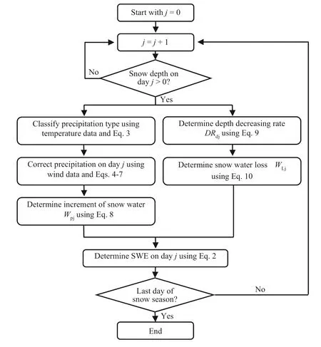
Fig. 2 Flowchart of the proposed algorithm to estimate the snow water equivalent (SWE)using snow depth and climatic data

(3) The daily increment of the SWE is estimated by summing up the snowfall and the rainfall that is absorbed by the snowpack.

(4) The daily snow water loss due to melting and/or evaporation is approximated by a decreasing rate multiplying the SWE on the previous day. The decreasing rate of the SWE is assumed to be equal to the decreasing rate of the snow depth after considering a daily densif ication rate of 5%. The rationale for this step and the use of 5% is explained in Sect. 3.4.

(5) The daily SWE is estimated by substituting the results of steps 3 and 4 in Eq. 2.

These evaluation steps are simple but associated with uncertainties as discussed in the following sections.

3.2 Adjustment for Precipitation Data

The gauge catch def iciencies have been investigated by different researchers, and many articles have been published on this subject (Larson and Peck 1974; Rasmussen et al.2012; Zhang et al. 2019). The precipitation gauge measurement error increases as the wind speed increases. The error is greater for solid precipitation (snow) than liquid precipitation (rain) because the trajectory of the snowf lake is easier to be inf luenced by the wind (Larson and Peck 1974; Yang et al. 1995; Goodison et al. 1998; Nitu et al. 2018). Consequently, it is necessary to determine whether the precipitation is rainfall or snowfall to account for the possible measurement errors. However, information on precipitation type is not available in the metadata acquired from CMA. To deal with this problem, in this study, the precipitation is classif ied as rainfall if there is no snow on the ground (ground snow depth is zero). When the ground snow depth measurement is greater than zero,the precipitation is treated as snowfall or mixed precipitation, depending on the climatic conditions. This mixed precipitation is represented by fractions of snowfall and rainfall, where the fractions could be evaluated as suggested by Ye et al. ( 2004) and Zhang et al. ( 2019). More specif ically, precipitation is classif ied as snowfall if the daily mean air temperature,Td , is lower than −2 °C, classif ied as rainfall ifTd is higher than +2 °C, and classif ied as mixed precipitation ifTdis between −2 °C and +2 °C.A linear function of temperature is adopted to estimate the fraction of precipitation that has fallen as snow,F s:

whereFsis equal to 1 whenTdis lower than −2 °C and 0 ifTd is higher than 2 °C. The fraction of precipitation that has fallen as rain,Fr , is equal to (1−Fs ).

The physical mechanisms that control the precipitation phase are much more complex than what the aforementioned model represents. Factors that aff ect the precipitation phase may include stability of the atmosphere, temperature lapse rate, the atmospheric humidity prof ile, and many others(Wang et al. 2019; Li et al. 2022). However, these factors are rarely adopted in applications since the implementation of these mechanisms would increase the model complexity and thus introduce more uncertainties (Wang et al. 2019).Consequently, the most popular methods to identify the precipitation type in practical applications are those based on near-surface air temperature (Li et al. 2022), which is also considered in this study.

Since this study is focused on the annual maximum values of the SWE, the uncertainty caused by the partition of precipitation may not be very important. This is because the mixed snow-rain events occur only in pre-winter or postwinter periods that are unlikely to aff ect the annual maximum values of the SWE. Therefore, neglecting the uncertainty in evaluatingF sis justif ied for assessing the snow load for structural design.

To determine the wind-induced error in measuring solid precipitation, the World Meteorological Organization(WMO) Solid Precipitation Measurement Intercomparison was initiated in 1985. Twelve countries, including China,participated and submitted complete data summaries for analysis in the intercomparison (Goodison et al. 1998). The intercomparison results were described in Yang et al. ( 1991)by using data from Tianshan glaciological station, China,from July 1987 to August 1991. The results indicate that,when compared to the double fence intercomparison reference, the average catch ratio (CR) for rain, rain and snow,wet snow, and dry snow is 95.82%, 89.03%, 83.62%, and 72.62%, respectively (Yang et al. 1991; Goodison et al.during the snow or rain event,U(m/s). According to Yang et al. ( 1991), it can be estimated using:for the rain, wherePscandPrcdenote corrected snowfall and rainfall, respectively;Pgis precipitation measured by the gauge;CRsandCRrare given in Eqs. 4 and 5, respectively,andFsis the fraction of precipitation that represents the snowfall given in Eq. 3. In Eqs. 6 and 7,Pwdenotes wetting loss that is caused by precipitation that is retained or stuck to the internal wall of the gauge and cannot be measured in precipitation observation. A value of 0.3 mm is taken forPw in this study (Yang et al. 1991; Ye et al. 2004; Zhang et al.2019). Trace precipitationPtcould not be measured by the gauge because of the resolution of the gauge, and a value of 0.1 mm is assigned for it when a trace precipitation event is recorded (Ye et al. 2004; Zhang et al. 2019).

Evaporation loss of precipitation measurements is ignored in this study as it is found that evaporation could be negligible for the Chinese Standard Precipitation Gauge(CSPG), which uses a funnel and a container (Ye et al. 2004;Ren and Li 2007).

3.3 Estimation of Snow Water Increment

A water-holding capacity of 3% (Zhou et al. 2013) is considered in this study. The maximum rainfall absorbed by the snowpack is then estimated by multiplying 0.03 and ground snow depth in mm. The increment of the SWE on dayj,ΔWPj, is then given by:

wheredjrepresents the snow depth on dayjin mm, andPscjandPrcjare corrected snowfall and corrected rainfall on dayj, respectively.1998). In general,CRdepends on the average wind speed

3.4 Estimation of Snow Water Loss

Water loss of snowpack is mainly caused by snowmelt,snow evaporation and/or snow sublimation. Male and Gray( 1975) indicated that the net amount of evaporation/condensation over a 24-h period during the snowmelt is generally negligible. But accurate estimation of the snowmelt is important for water resources management and f lood risk assessment. Thus, the modeling of the snowmelt process has long been studied in hydrology (Anderson 1968;Male and Gray 1975; Kustas et al. 1994; Boudhar et al.2016). Snowmelt models are mainly based on the energy balance equation of the snowpack (Kondo and Yamazaki 1990; Tarboton and Luce 1996; Zeinivand and De Smedt 2010). A simplif ied model such as the degree-day model has also been developed and applied (Johannesson et al.1995; Braithwaite and Zhang 2000).

Unfortunately, the required input data and/or model parameters for the energy balance equation or degreeday model are not reported for ordinary meteorological stations. So rather than use the degree-day model or the energy balance model to estimate the SWE, the proposed algorithm in this study assumed that snow water loss is proportional to the reduction of snow depth.

Note that there is a densif ication process in the snowpack due to gravity, wind, precipitation, and temperature gradient (Yang, Zhang et al. 1992; Sturm and Holmgren 1998). Therefore, a decrease in snow depth does not necessarily imply a reduction in the SWE. Sturm and Holmgren( 1998) showed that the average densif ication rate of snow for regions classif ied as Maritime, Tundra, and Taiga is 1.31, 0.24, and 0.57 kg/m3/d, respectively. The densif ication rate for freshly fallen snow is relatively higher because the fresh snow is looser and compacts more easily.Yang, Zhang et al. ( 1992) indicated that the snow density of fresh snow increases by about 5% on the second day.Considering the typical average density of 70–110 kg/m 3 for fresh snow, the corresponding densif ication rate is 3.5–5 kg/m 3 /d. This is close to the 4 kg/m 3 /d given by Wei et al. ( 2001). However, these values are much lower than the 9.6 kg/m 3 /d given by Chen et al. ( 2011). The wide range of snow densif ication rates indicates that snow densif ication varies signif icantly and is complicated to predict. As a simplif ication, an average densif ication rate of 5% is adopted in this study. This results in a reduction of approximately 5% in snow depth each day with the SWE remaining the same as the previous day.

Densif ication is assumed to last for 10 days after the occurrence of the snowfall event, and the f inal density is equal to 1.05 10 (or 1.63) times that of the original density.For a typical fresh snow density of about 70–110 kg/m 3 ,the corresponding f inal density after densif ication is then estimated to be 115–180 kg/m 3 , which is consistent with the observed values in China (Mo et al. 2016; Mo, Cao et al.2022). Based on this assumption, the decreasing rate of snow depth on dayj,DRdj, is given by the following equation:

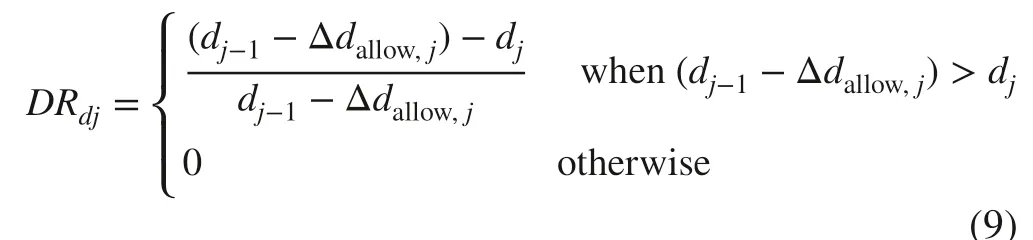
wheredj−1anddjdenote ground snow depth on dayj−1 and dayj, respectively, and Δdallow,jis the allowance of snow depth reduction on dayjthat is the summation of potential depth reduction for all snow events within 10 days. Snow water loss on dayj, ΔWLj , is then approximated by applying the decreasing rate to the SWE on the previous day:

In addition, the criterion for the limiting values of the density that was applied to the original snow data is also applied to the estimated SWE. That is, the associated snowpack bulk density that is calculated by dividing the derived SWE by the recorded ground snow depth for the same day should not be less than 50 kg/m 3 or greater than 400 kg/m 3 .

4 Results and Discussion

Based on the proposed procedure, the daily SWE was estimated from the ground snow depth and climatic data for the considered stations shown in Fig. 1 b. The estimated daily SWE, as well as the annual maximum SWE, are compared to the measured ones to validate the proposed algorithm. The snow hazard map for northeastern China is then developed using the measured and calculated SWE.

4.1 Comparison of the Calculated and Measured Snow Water Equivalent

Examples of such a comparison are shown in Fig. 3 for four representative sites identif ied in Fig. 1 b, where the data points represent the daily SWE for all available years(1971–2018) for the corresponding station. When plotting the f igures, data points that are associated with 0 value in both the calculated and measured SWE are eliminated. Figure 3 shows that the calculated and measured SWE values are in good agreement as they are concentrated near the diagonal line. Their correlation coeffi cients,r, are greater than 0.83, and the bias ranges from 0.2 to 3.1mm.

Diff erences between the calculated SWE and SWE measurements could also be observed. These diff erences could be attributed to the following f ive causes:

Fig. 3 Comparison of the calculated daily snow water equivalent (SWE) and SWE measurements in northeastern China: a Site 1(2,424 data points); b Site 2 (2,129 data points); c Site 3 (2,119 data points); and d Site 4 (1,818 data points). Locations of the four sites are indicated in Fig. 1 b.

(1) The diff erence or gap between the measured SWE and precipitation. In some cases, the gap between recorded precipitation and the SWE is too large to be closed by the correction of the precipitation data. For example,at Site 2, the measured SWE for 30 November and 5 December 1987 is 40 and 51 mm, respectively, which indicates that a total of 11 mm of SWE due to snowfall occurred within the f ive days. But the corresponding recorded precipitation within these f ive days was only 0.1 mm and two trace precipitation events, or only 0.6 mm in total after wetting loss correction and trace precipitation correction. This leaves a large diff erence between the precipitation and the measured SWE.

(2) The criteria for the SWE measurements. The SWE is measured following specif ied criteria (that is, every 5 days if the ground snow depth is greater than 5 cm;additional measurement is carried out only if the depth increment due to new snowfall exceeds 5 cm). If ground snow depth is less than 5 cm, no SWE is reported even though the actual SWE may not be zero. The absence of SWE measurement, in this case, will certainly cause bias between the recorded and the calculated SWE.

(3) The uncertainties caused by the determination of the snow fraction in total precipitation. The variability in the diff erence between the calculated and the measured SWE could be caused by the uncertainty in the calculated fraction of snowfall (see Eq. 3). Part of this uncertainty is attributed to the fact that the continuous air temperature variation data during a day is unavailable, and only daily maximum, minimum, and average temperatures are reported. For example, a snowfall of 15 mm was recorded on 4 April 1999 for Site 3; the average temperature for that day is 0.6 °C, resulting in aFsof 0.4 according to Eq. 3. The precipitation that fell as snow is estimated to be only 5.4 mm in this case,or 5.8 mm after correction, which is much less than the measured SWE of 15 mm. Such a discrepancy could be reduced or eliminated if the continuous air temperature was recorded, reported, and used to calculate the SWE.

(4) The uncertainties caused by the precipitation correction model shown in Eqs. 4– 7. The sampling frequency of climatological elements such as wind speed and precipitation is very low. This could aff ect the calculated (that is, corrected or adjusted) precipitation amount. This problem could only be investigated using data with a higher sampling frequency, which was unavailable for this study.

(5) The uncertainties caused by the estimation of snow water loss. The estimation model for snow water loss given by Eqs. 9 and 10 assume that the snow water loss is proportional to the decrease of snow depth upon the consideration of a densif ication rate of 5%. However,as pointed out in Sect. 3.4, snow densif ication is a complicated process and varies signif icantly with time and location. The use of a single 5% value of the densif ication rate will bring uncertainties to the estimation of snow water loss and further to the estimation of the SWE.

The above observations suggest that a better estimate of the daily SWE may be obtained if more detailed measurements of the climatological elements for a site of interest are reported and used with the proposed algorithm.

4.2 Comparison of the Calculated and Measured Annual Maximum Snow Water Equivalent

This section presents the comparison of the annual maximum SWE extracted from the calculated and measured SWE values. The comparison is focused on the probability distribution and theT-year return period value of the annual maximum SWE.

For each of the 57 meteorological stations depicted in Fig. 1 b, a probability distribution f itting was carried out for the extracted annual maximum SWE. For the distribution f itting, the Gumbel distribution and the lognormal distribution were considered as the candidate probability distribution.The consideration of the Gumbel distribution is justif ied since it is recommended by the Chinese structural design code (MOHURD 2012) and used for the structural design code calibration for other jurisdictions (Bartlett et al. 2003;BSI 2003; NRCC 2015; Hong et al. 2021; Mo, Cao et al.2022). The lognormal distribution is considered because it is preferred for the annual maximum ground snow depth or SWE (Ellingwood and Redf ield 1983; ASCE 2016; Mo et al.2016; Mo, Ye et al. 2022).

The Gumbel distribution can be written as (Coles 2001):wheremlnxand σlnxare the distribution parameters that represent the mean and standard deviation of ln(x), respectively,and Ф( ) denotes the standard normal distribution function.

To identify the preferable probability model for the annual maximum SWE, the Akaike Information Criterion with a small sample size (AICc) (Burnham and Anderson 2003) is considered:

wherekis the number of model parameters,nis the sample size, andLis the maximum likelihood of the considered model. The preferred model among the candidate models is the one that leads to the lowest AICc value. The distribution f itting results indicate that the Gumbel distribution and lognormal distribution are preferred by 18 and 39 stations,respectively, if the measured SWE is considered, and by 9 and 48 stations, respectively, if the estimated SWE is considered. It was observed that in many cases, the diff erences in AICc for the considered two models are not very large. The preference for the lognormal distribution is consistent with the observation made by Mo et al. ( 2016), which indicated that the lognormal distribution is preferable for the annual maximum SWE or annual maximum ground snow depth from about two-thirds of the sites considered in their study.

Since there is no clear spatial trend on the preferred distribution of the SWE, the preferred lognormal distribution is considered in the following. Moreover, since the use of the method of L-moments (Hosking and Wallis 1997) is recommended in the literature, it is used to f it the annual maximum SWE. The empirical and the f itted distributions for the four representative sites identif ied in Fig. 1 b are presented in Fig. 4.

Figure 4 indicates that the empirical and f itted probability distributions of the annual maximum SWE extracted from the calculated SWE match well with those of the annual maximum extracted from the measured SWE, especially for Sites 1 and 4. The diff erences between the empirical distributions based on the calculated and measured data are appreciable. As has been pointed out in the previous section,the diff erences are attributed to various reasons and could be reduced if more detailed measurements of the climatological elements for a site of interest are reported and used with the proposed algorithm..

To better quantify the impact of using the SWE calculated using the proposed algorithm in estimating the snow hazard, the 50-year return period value of the annual maximum SWE,s50, for the considered four sites in Fig. 1 b, was calculated based on both the calculated and measured SWE.The calculated values are shown in Table 1. Note thats50shown in the table is presented in kPa, which is converted from mm by considering a water density of 1,000 kg/m 3 and a gravitational acceleration of 9.8 m/s 2 . The comparison indicated that the relative diff erence–that is, (s50based on the calculated SWE–s50based on the measured SWE) /(s50based on the measured SWE)–is site-dependent; the absolute value of the relative error is less than about 17%for the four representative sites.

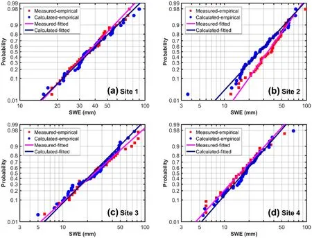
Fig. 4 Fitted lognormal distribution of the annual maximum snow water equivalent (SWE) for the four representative stations in northeastern China

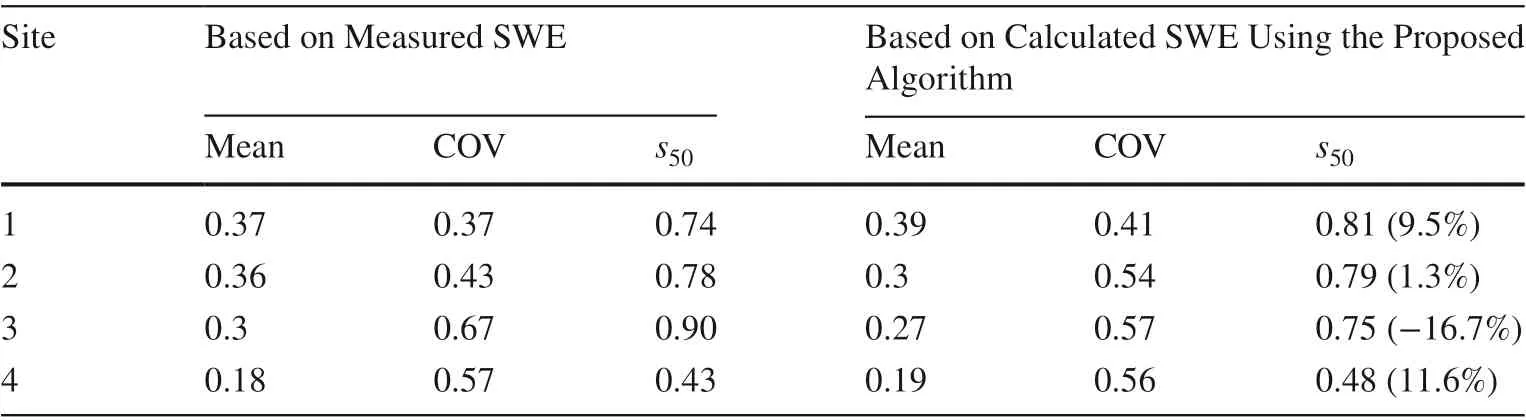
Table 1 Statistics of the annual maximum snow water equivalent (SWE) (kPa) for the four representative stations in northeastern China (value within the bracket represents the relative error)

The analysis that is carried out for the four representative sites is repeated for each of the 57 meteorological stations depicted in Fig. 1 b. The obtained results are shown in Fig. 5 a. The f igure indicates that the proposed algorithm estimatess50fairly well for locations withs50less than about 0.8 kPa, but underestimates thes50for locations wheres50is higher than about 0.8 kPa. More specif ically, a histogram of the estimation error,Err, (Fig. 5 b) shows that the distribution of the error is left-skewed, implying that the proposed algorithm tends to underestimate thes50in general. A correction to the estimateds50is desired to eliminate such a trend.

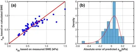
Fig. 5 Comparison of s 50 estimated by considering the measured snow water equivalent (SWE) and the SWE estimated based on the proposed algorithm: a Comparison of s 50 ; b Histogram of the estimation error in estimated s 50 .

Fig. 6 Variation of estimation error in s 50 with statistics of ground snow: a Variation of estimation error with s 50 estimated from the measured snow water equivalent (SWE); b variation of estimation error with d 50 (50-year ground snow depth).

For the purpose of correcting the estimateds50, attempts are made to plotErrversus the 30-year normal of winter precipitation (December, January, February), normal of maximum winter wind speed, and normal of mean coldest month temperature. Unfortunately, no trend is observed. However,whenErris plotted versuss50estimated from the measured SWE (Fig. 6 a), an apparent decreasing trend fors50greater than about 0.6 kPa, and an increasing trend fors50 less than 0.6 kPa could be observed. Although the reasons for these trends are not clear in this study–and whether the trends are applicable to other regions requires further investigation when snow data for other regions become available–the trends provide a basis for the correction of the estimateds50from a practical point of view, at least for the region of interest.

Since the proposed algorithm is designed for stations where SWE measurements are not available, the correction is made according to 50-year ground snow depth,d50, instead ofs50. The variation ofErrwithd50is depicted in Fig. 6 b.Comparing Fig. 6 a and b shows that the trends ofErrin Fig. 6 b are quite similar to those in Fig. 6 a. Regression analysis is carried out to modelErrand it is found that a polynomial of order 2 is adequate to model the error:

where μEis the modeled value ofErr(see the red line in Fig. 6 b), ε is the residual of the regression, andErrandd50are in the unit of kPa and m, respectively. The regression residual ε is normally distributed (Fig. 7 b). The correcteds50,s50,cor, could then be expressed as:

wheres50,calis thes50estimated from the calculated SWE.Similar to Fig. 5 a, the corrected estimation ofs50is compared tos50 estimated from the measured SWE in Fig. 7 a.The f igure shows that the corrected estimation ofs50 follows the diagonal line fairly well, implying that a good estimation ofs50was obtained. It also indicates that the correction improves the estimation effectively when compared to Fig. 5 a. The estimation error of the correcteds50is the same as the residual shown in Fig. 7 b, which could be assumed to be normally distributed.

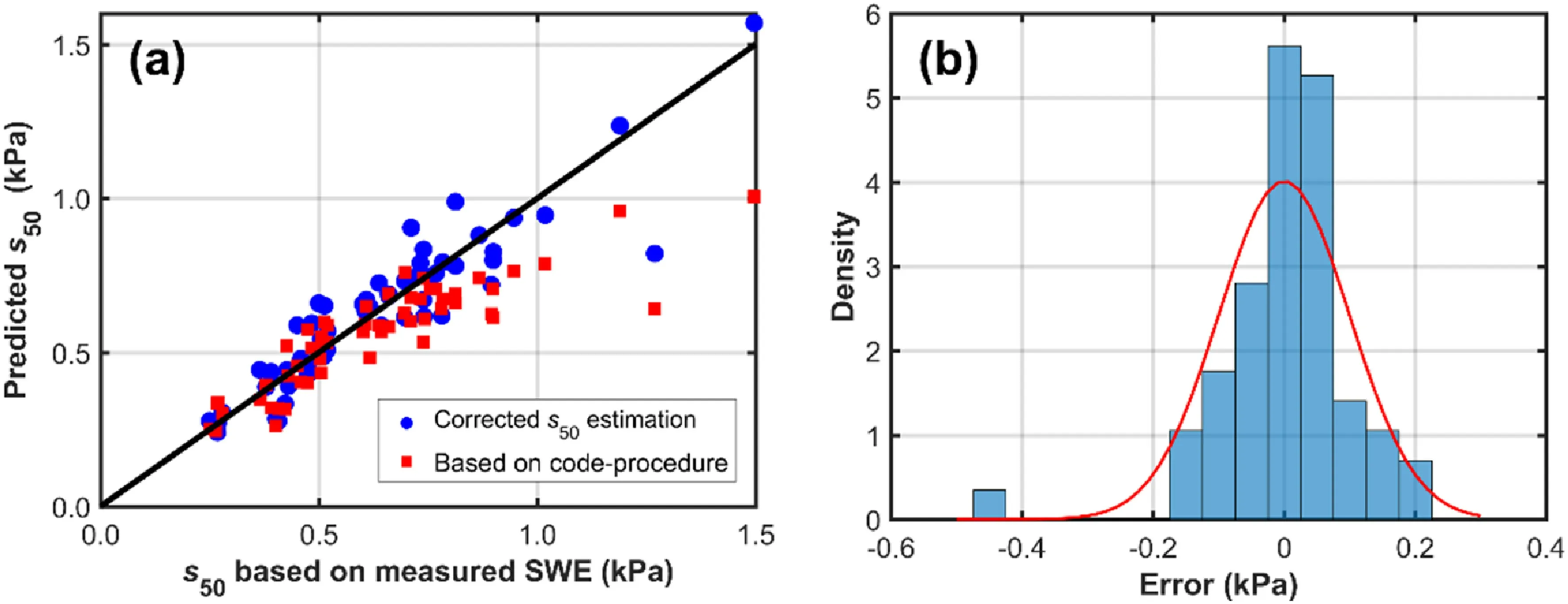
Fig. 7 Comparison of corrected s 50 with that estimated by considering the measured snow water equivalent (SWE): a Comparison of s 50 ; b Histogram of the estimation error in corrected s 50 .

To see the ground snow load in the context of the structural design code making, it is noted that the Chinese load code for the design of building structures (MOHURD 2012)recommends thats50could be evaluated based on the average snowpack density and the 50-year annual maximum ground snow depth when SWE measurements are not available:

where ρavgis the applicable average snowpack density for the considered site, which is equal to 150 kg/m 3 for northeastern China,g= 9.8 m/s 2 is the gravitational acceleration, andd50is the 50-year return period value of the annual maximum snow depth, which is calculated by assuming that the annual maximum ground snow depth is Gumbel distributed (as recommended in the code). The obtaineds50 by using Eq. 16 is also included in Fig. 7 a for the considered sites. The f igure indicates that the error of the estimateds50based on the SWE evaluated using the proposed algorithm, in general,is smaller than that suggested by the code procedure. This suggests that for sites without measured SWE, the use of the proposed algorithm to evaluate the SWE can result in a more accurate estimate ofs50.

4.3 Mapping the Snow Hazard Using the Measured and Calculated Snow Water Equivalent

To illustrate the application of the proposed algorithm in snow hazard mapping, f irst, the calculateds50–by using the measured SWE for the 57 considered meteorological stations depicted in Fig. 1 b–is presented in Fig. 8 a to map the snow hazard. Second, the calculateds50for the same stations but considering the SWE evaluated based on the proposed algorithm is presented in Fig. 8 b. Third, to improve the spatial coverage,s50–for all stations shown in Fig. 1 a–was estimated by using the SWE evaluated based on the proposed algorithm. The obtaineds50 was then mapped and is shown in Fig. 8 c. Fourth, the snow hazard was mapped as shown in Fig. 8 d by usings50, which was estimated based on the measured SWE if the measurements are available from a station; otherwise it was estimated based on the SWE calculated using the proposed algorithm. Finally,s50–calculated according to the structural design code-suggested practice(see Eq. 16)–was mapped in Fig. 8 e. Four major observations could be drawn from Fig. 8:

(1) The spatial trends and the magnitudes of the mappeds50 estimated based on the measured SWE (Fig. 8 a) and based on the calculated SWE by applying the proposed algorithm (Fig. 8 b) are consistent except the outlier located in the central-east of the region, where thes50is underestimated signif icantly by the proposed algorithm.

(2) The use ofs50by considering all stations shown in Fig. 1 a improves the granularity of the mapped hazard(by comparing Fig. 8 b and c), indicating the usefulness of applying the proposed algorithm in augmenting the SWE data.

(3) The use ofs50estimated based on the measured SWE and the calculated SWE, when the measured SWE is unavailable, leads to a snow hazard map with ref ined resolution. A comparison of Fig. 8 a and d indicates that the consideration of extra stations could reduce the inf luence of outliers on the hazard map.

Fig. 8 Snow hazard map for northeastern China: a Using s 50 estimated based on measured snow water equivalent (SWE) for the 57 stations; b Using s 50 estimated based on the calculated SWE for the 57 stations; c Using s 50 estimated based on the calculated SWE for all 99 stations depicted in Fig. 1 a; d Using s 50 estimated based on the calculated and measured SWE (when available); and e Using s 50 estimated based on code-suggested procedure (see Eq. 16).

(4) Comparison of Fig. 8 a–e indicates that the use of the code-recommended approach results in the mapped hazard that diff ers from those obtained based on the measured SWE or calculated SWE. It indicates that the code-recommended approach (MOHURD 2012) should be reassessed.

5 Conclusions

For snow hazard-prone regions, the estimation of extreme ground snow loads for locations where only ground snow depths are available is of great importance. Given the ground snow depth alone, this estimation is challenging since the snowpack bulk density is uncertain and with signif icant temporal and spatial variability. By considering the relationship between the snow water equivalent (SWE) and precipitation,a new algorithm or procedure is proposed to estimate the SWE (or ground snow load). Using the proposed algorithm,the ground snow depth records, and the temperature, precipitation, and wind speed records, the SWE (or ground snow load) history was calculated and compared with the recorded SWE values for 57 locations in northeastern China. Also,an analysis of the 50-year return period value of the ground snow load was carried out based on the measured SWE, the calculated SWE using the proposed algorithm, and the procedure recommended by the Chinese load code. Snow hazard maps were developed based on the estimateds50. Three main conclusions can be drawn from the numerical results:

(1) In general, the SWE obtained by using the proposed algorithm agrees well with the measured SWE.

(2) The spatial trends and the magnitudes of the mappeds50estimated based on the measured SWE and based on the calculated SWE by applying the proposed algorithm are consistent, indicating the usefulness of applying the proposed algorithm in augmenting the SWE data.

(3) The error analysis and comparison of the mapped snow hazards indicate that the code-recommended approach should be reassessed by the committee that reviews the snow load for the load code (MOHURD 2012) since it leads to the 50-year return period value of the snow load deviating signif icantly from that estimated based on the measured SWE.

AcknowledgmentsFinancial support from the National Natural Science Foundation of China (Grant Nos. 51808169 and 51927813), and the Fundamental Research Funds for the Central Universities (Grant No. HIT. NSRIF. 2020083) are gratefully acknowledged.

Open AccessThis article is licensed under a Creative Commons Attribution 4.0 International License, which permits use, sharing, adaptation, distribution and reproduction in any medium or format, as long as you give appropriate credit to the original author(s) and the source,provide a link to the Creative Commons licence, and indicate if changes were made. The images or other third party material in this article are included in the article’s Creative Commons licence, unless indicated otherwise in a credit line to the material. If material is not included in the article’s Creative Commons licence and your intended use is not permitted by statutory regulation or exceeds the permitted use, you will need to obtain permission directly from the copyright holder. To view a copy of this licence, visit http:// creat iveco mmons. org/ licen ses/ by/4. 0/.